Executive Summary

RMA will be an optional model within IFRS 9 for net interest rate repricing risk¹ in dynamic, open portfolios (for example, where new deposits or loans are continually added and existing positions mature or reprice). The IASB also proposes withdrawing the IAS 39 macro hedge requirements (and the IFRS 9 option to apply them) and adding related IFRS 7 disclosures.

Compared with current IFRS 9 hedge accounting, RMA shifts from item-level hedges to portfolio net-position accounting, better aligned to typical banking book features (for example, non-maturity deposits and pipeline exposures). Compared with IAS 39 macro hedging (including the EU carve-out), it replaces bucket-based rules and carve-out reliefs with a principles-based net exposure model.

At a high level, the RMA model works as follows:

• Set the target: the entity specifies how much net interest rate risk it aims to mitigate over time, within defined risk limits and not exceeding the net exposure in each time band (bucket). The target can be updated prospectively as the balance sheet evolves.
• Link to derivatives: external interest rate derivatives can be designated. The model uses benchmark derivatives (hypothetical instruments with zero fair value at inception) to represent the risk the entity intends to mitigate.
• Recognize an adjustment: a risk mitigation adjustment is recognized on the balance sheet. It equals the lower of (I) the cumulative value change of the designated derivatives and (II) the cumulative value change of the benchmark derivatives. Any remaining derivative gains or losses (and any ‘excess’ adjustment) go to profit or loss.
• Release to earnings: the risk mitigation adjustment is released to profit or loss as the underlying repricing effects occur.

RMA is a meaningful step toward aligning accounting with how banks manage banking-book interest rate risk in dynamic, open portfolios. At the same time, the ED leaves important practical questions open, notably on benchmark-derivative construction, operation of the excess test, and the level of data, systems, and governance needed for ongoing application.

After the 31 July 2026 deadline, the IASB will review comment letters and fieldwork feedback and decide whether further deliberations are needed, so finalization is likely to take several years. Even once the IASB issues a final standard, application in the EU would still depend on completion of the endorsement process (EFRAG advice, Commission adoption, and Parliament/Council scrutiny).

Introduction

On December 3^rd, 2025, the IASB published the ED proposing RMA for interest rate risk in dynamic portfolios. RMA is the result of the IASB’s long-running efforts on accounting for dynamic interest rate risk management, previously referred to as DRM. RMA focuses on repricing risk, which is the interest rate risk that arises when the timing and amount of repricing differ between assets and liabilities.

The aim is to better reflect how banks manage interest rate risk in the banking book at a portfolio level, an area where existing hedge accounting requirements have long been seen as difficult to apply in a way that aligns with real-world balance sheet management.

The IASB presents RMA as a step forward, to better reflect how banks manage interest rate risk in the banking book at a portfolio level, an area in which existing IAS 39 and IFRS 9 hedge accounting requirements have long been viewed as difficult to apply in a way that aligns with real-world, dynamic balance sheet management. In the IASB’s view, RMA is intended to improve that alignment, increase transparency about the effects of repricing-risk management on future cash flows, strengthen consistency between what is managed and what is eligible for accounting treatment, and recognize in the financial statements the extent to which repricing risk has actually been mitigated and the related economic effects.

This article provides a structured overview of the proposed RMA model and its key mechanics. Throughout the article, Zanders provides practical insights on the impact on entities, highlighting the key areas that will shape implementation challenges and accounting results. These insights draw on Zanders' 2025 survey on interest rate risk management and hedge accounting, as well as analysis of stakeholder feedback such as EFRAG's draft comment letter². The practical implications will depend in part on the outcome of field testing.

Overview of RMA

The model components and their relationships are presented in Figure 1 below:

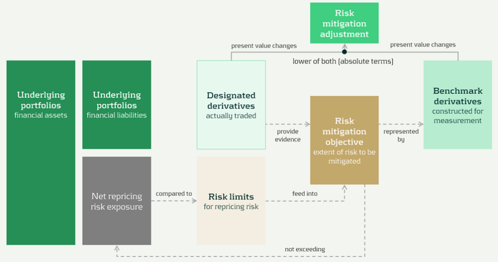
Figure 1: RMA model component overview (source: IASB ED – Snapshot, December 2025)

The RMA model is built around a small set of linked building blocks that start with the bank’s balance-sheet exposures and end with the accounting adjustment that reflects risk management in the financial statements:

• Underlying portfolios: the managed portfolios that expose the entity to repricing risk.
• Net repricing risk exposure: the net position created by the interaction of asset and liability repricing profiles (i.e., the aggregate repricing mismatch the bank is exposed to).
• Risk limits: the bank’s risk appetite and constraints for the managed exposure. In the model, these limits act as an important boundary.
• Risk mitigation objective: the clearly articulated target for how much of the net repricing risk exposure management intends to mitigate (within risk limits). This objective is the central anchor in the model.
• Designated derivatives: the derivatives the bank trades to achieve the risk mitigation objective.
• Benchmark derivatives: hypothetical derivatives constructed to represent the risk mitigation objective for measurement purposes. They translate the objective into a measurable reference profile against which fair value changes can be assessed.
• Risk mitigation adjustment: the accounting output of the model, which is the lower of the change in fair value of the benchmark derivatives and the designated derivatives (in absolute terms).

The section headers contain the relevant paragraph of the ED. The body of the text refers to the ED amendments to IFRS 9 [7.x.), application guidance [B7.x.x), basis for conclusions [BCx), and illustrative examples [IEx), and amendments to IFRS 7 [30x).

Speak to a Zanders expert

Objective and scope [ED 7.1]

IFRS 9 hedge accounting improves alignment for many strategies, but it does not fully capture dynamic, open-portfolio (macro) management of banking book repricing risk—where entities manage interest rate risk of net open positions rather than hedging individual instruments. The RMA model is intended to reflect this more directly and reduce reliance on proxy hedges that can obscure transparency and comparability.

The objective and scope of RMA can be summarized as follows:

• Objective: RMA is, like current hedge accounting under IAS 39 and IFRS 9, an optional model within IFRS 9. The objective is to reflect the economic effect of risk management activities and improve transparency by explaining why and how derivatives are used to mitigate repricing risk and how effectively they do so —bringing reporting closer to actual interest rate risk management practices [7.1.3]. It is the IASB’s intention to withdraw the requirements in IAS 39 for macro hedge accounting and the option in paragraph 6.1.3 of IFRS 9 to apply the requirements in IAS 39 to a portfolio hedge of interest rate risk.
• Scope/eligibility: An entity may apply RMA if, and only if, all of the following are met [7.1.4]:
  • Business activities give rise to repricing risk through the recognition and derecognition of financial instruments that expose the entity to repricing risk.The risk management strategy specifies risk limits within which repricing risk, based on a mitigated rate, is to be mitigated, including the time bands and frequency.
  • The entity mitigates repricing risk arising from underlying portfolios on a net basis using derivatives, consistent with the entity’s risk management strategy.
• Application discipline: RMA is applied at the level where repricing risk is actually managed and requires robust formal documentation (strategy, mitigated rate, mitigated time horizon, risk limits, and methods for determining exposures and benchmark derivatives) [7.1.6, 7.1.7].

Key considerations and insights

1. Objective: RMA’s objective to reflect the economic effect of risk management activities may not always coincide with eliminating accounting mismatches (as suggested by other key considerations and insights later in this article). For example, EFRAG’s draft comment letter agrees that faithful representation is a key objective and could improve current accounting, for example, by reducing reliance on proxy hedging. However, it questions whether this should be treated as equally important as eliminating accounting mismatches. This aligns with the concerns expressed around the impact on the hedge effectiveness by several European banks in Zanders’ 2025 survey on interest rate risk management and hedge accounting3, while more than 80% of the participants assessed its effectiveness under the current hedge accounting approach as acceptable.

Net repricing risk exposure [ED 7.2]

Entities are required to determine a net repricing risk exposure across underlying portfolios by aggregating repricing risk exposure using expected repricing dates, within each repricing time band as required to be defined in formal documentation.

Key requirements include:

• Eligible items Underlying portfolios can include [7.2.1; B7.2.1–B7.2.2]:
  • Financial assets measured at amortized cost or FVOCI,
  • Financial liabilities at amortized cost, and,
  • Eligible future transactions that may result in recognition/derecognition of such items.
• Portfolio view and behavioral profiles: Items that may not show sensitivity on an individual basis (for example, demand deposits) can still contribute to repricing risk on a portfolio basis. A stable ‘core’ portion may be treated as behaving like longer-term funding if supported by reasonable and supportable assumptions and consistent with risk management [B7.2.2].
• Expected repricing dates and time bands: Expected repricing dates must be measured reliably using reasonable and supportable information (including behavioral characteristics such as prepayments and deposit stability). Time bands and risk measures (e.g., maturity gap or PV01) must be consistent with actual risk management [7.2.5–7.2.9; B7.2.10–B7.2.16].
• Equity modelling as a proxy: Own equity is not eligible for inclusion in underlying portfolios, but the model acknowledges that some entities assess repricing risk from cash/highly liquid variable-rate assets only to the extent they are ‘funded by equity’. If internal equity modelling (e.g., replicating portfolios) is used for risk management, it can serve as a proxy to determine how much of those exposures are included in net repricing risk exposure [B7.2.17; IE184-IE191].

Key considerations and insights

2. Eligibility: RMA aims to reflect net repricing risk management, but eligibility rules can make the net repricing risk exposure only a partial proxy for the position Treasury actually manages. For example, banks might include fair value through profit or loss (FVTPL) items for interest rate risk management but these are not allowed as underlying items in the net repricing risk exposure (also noted by EFRAG).

3. Risk management by time bands (1/2): RMA requires a risk mitigation objective based on the net repricing risk exposure determined for each repricing time band, but it is unclear how entities that do not manage their interest rate risk across time bands would then apply the RMA model, as noted by EFRAG.

4. Risk management by time bands (1/2): RMA requires the same risk measure (e.g., maturity gap or PV01) for all exposures within each repricing time band [B7.2.13], but banks’ risk management practice might deviate from this.

5. Equity treatment: RMA introduces an equity proxy approach that allows partial inclusion of variable-rate assets based on modelled equity, viewing equity as residual and ineligible for direct inclusion. This is an addition compared to the DRM staff papers. Banks' risk management practices might treat equity differently (e.g., by modelling it).

Designated derivatives [ED 7.3]

Under RMA, banks can designate external derivatives (e.g., interest rate swaps, forwards, futures, options) used to manage net repricing risk as hedging instruments. Eligible derivatives are generally consistent with IFRS 9. All designated derivatives collectively mitigate the net portfolio risk and remain recognized at fair value.

Eligibility depends on the following items:

• Mitigation: Derivatives can only be designated to the extent that they mitigate the net repricing risk exposure [7.3.6].
• External counterparty: Derivatives must be with a counterparty external to the reporting entity. Intragroup derivatives may qualify only in the separate or individual financial statements of the relevant entities, and are not eligible in the consolidated financial statements of the group [7.3.4].
• Designate once: Derivatives already in a hedging relationship for interest rate risk in accordance with Chapter 6 of IFRS 9 are not eligible [7.3.5].
• Options: Written options are generally excluded, unless part of a net written option position that offsets a purchased option, resulting in a net purchased position overall [7.3.2(a), 7.3.3].

Banks can designate derivatives in full or in part (e.g., designating 80% of a swap if only that portion manages interest rate risk), but the selected portion must align with the documented risk mitigation objective.

Once derivatives are designated, they can only be removed from RMA if they are no longer held to mitigate the net repricing risk exposure under the entity’s risk management strategy.

Key considerations and insights

As the EFRAG comment letter notes: 6. Options and off-market derivatives: Further guidance is needed on how to treat options (for example, time value) and off-market derivatives (non-zero initial fair value) within the designation mechanics.

7. De-designation: The ED does not allow voluntary de-designation, but banks often manage changes by entering into offsetting trades rather than settling existing positions.

Risk mitigation objective [ED 7.4]

The risk mitigation objective is the bridge between risk mitigation intent and what’s actually executed: it sets how much net repricing risk exposure the entity aims to mitigate within risk limits [7.4.2]. The benchmark derivatives and consequently the risk mitigation adjustment are built from this risk mitigation objective (see next sections), enabling partial hedging while avoiding objectives that aren’t supported by actual designated hedges. [ED 7.4.1, B7.4.2–B7.4.3].

Key requirements:

• Evidence-based: The objective must be consistent with the repricing risk mitigated by designated derivatives—it’s a matter of fact, not a free choice. [ED 7.4.1, B7.4.2–B7.4.3]
• Absolute, not proportional: It’s stated as an absolute amount of risk (e.g., PV01), not ‘X% of each instrument’ [B7.4.2].
• Capped by exposure: It cannot exceed net repricing risk exposure (overhedge) in any time band [7.4.1, B7.4.2–B7.4.3].
• Measurement basis: The risk mitigation objective should be set using the same risk measure (e.g., DV01) used to quantify exposure [ED B7.4.1].

Key considerations and insights

8. Repricing time bands are a key design choice: the risk mitigation objective is specified and capped by the net repricing risk exposure in each time band. Executing (and designating) hedges in neighboring tenors (a common practice) can create residual P&L volatility, because only the portion aligned to that time band’s net repricing risk exposure is reflected in the risk mitigation adjustment.

9. Degree of freedom risk limits: While RMA imposes strict alignment requirements between net repricing risk exposure, risk mitigation objective, and designated derivatives on measures and time bands, entities retain strategic flexibility on risk limits. Risk limits do not need to be specified per time band [B7.4.6], allowing entities to set overarching frameworks rather than granular constraints.

Benchmark derivatives [ED 7.4]

Benchmark derivatives are introduced to measure hedge performance: modelled (hypothetical) derivatives that are not executed and not recognized on the balance sheet, but are constructed to replicate the timing and amount of repricing risk captured in the risk mitigation objective, as presented in Figure 1 above and Figure 2 below.

In practice, the benchmark derivative is designed to mirror the bank’s target risk position (e.g., a swap profile that matches the repricing ‘gap’ being mitigated), so its fair value movement represents how the net repricing risk exposure would change when interest rates move. If an entity intends to mitigate 70 of the 100 units of repricing risk in the 9-year time band by a 10-year swap, the benchmark derivative is based on 70 units and 9 year maturity [B7.4.8].

Benchmark derivatives should have an initial fair value of zero based on the mitigated rate [7.4.5]. These benchmark derivatives are therefore similar to the hypothetical derivative used in cash flow hedging [B6.5.5–B6.5.6 of IFRS 9].

Key considerations and insights

10. Operational burden (1/3) – benchmark derivatives: RMA intentionally separates designated derivatives from benchmark derivatives (constructed to start at zero fair value at the mitigated rate), so they won’t always share the same terms. This can become operationally heavy, as also noted by EFRAG.

Risk mitigation adjustment [ED 7.4]

The risk mitigation adjustment is the accounting output of the model and is presented as a single line item on the balance sheet (asset or liability). At each reporting date (so not necessarily the hedging date), the entity compares the cumulative fair value change of all designated derivatives with the cumulative fair value change of all the benchmark derivatives, and recognizes the lower of those two amounts (in absolute terms) [7.4.8] as the risk mitigation adjustment. That balance sheet adjustment is the mechanism that offsets the designated derivatives’ fair value changes in profit or loss; any remaining gain or loss (i.e., the portion not captured by the lower-of) is recognized directly in profit or loss as residual volatility/ineffectiveness [7.4.9].  This is visualized in Figure 2 below.

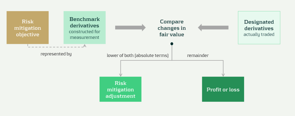
Figure 2 Recognition and measurement of risk mitigation adjustment (source: IASB ED – Snapshot, December 2025)

The 'lower of' mechanism ensures the risk mitigation adjustment never exceeds what's actually supported by either (I) the designated derivatives or (ii) the net exposure being hedged. This prevents over-recognition of hedging effects.

The risk mitigation adjustment is then recognized in profit or loss over time on a systematic basis that follows the repricing profile of the underlying portfolios [7.4.10], so the hedging effect shows up in the same periods in which the hedged repricing differences affect earnings.

Key considerations and insights

11. Operational burden (2/3) – risk mitigation adjustment: Heavy tracking requirements (including effects of settling vs offsetting trades), unclear calculation granularity, and complexity over time as the risk mitigation adjustment can flip between debit and credit, as noted by EFRAG.

12. RMA as a balance sheet item: The RMA model creates a separate balance sheet asset/liability (unlike current hedge accounting that adjusts hedged items or uses equity), introducing uncertainty around whether this item will attract RWA or require capital deductions until regulators provide guidance.

Prospective (RMA excess) and retrospective (unexpected changes) testing [ED 7.4]

RMA is designed to keep the accounting mechanics anchored to the net repricing risk exposure that actually remains in the underlying portfolios over time. Two tests can lead to changes to the risk mitigation adjustment. These tests are visualized in Figure 3 below, indicated by ① and ②.

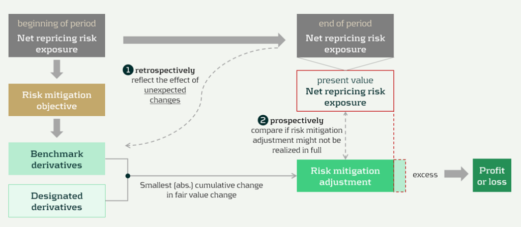
Figure 3 Risk mitigation adjustment and prospective and retrospective testing (source: IASB ED – Snapshot, December 2025)

The two tests are:

1. Benchmark adjustments for unexpected changes (retrospectively): First, benchmark derivatives must be adjusted when unexpected changes in the underlying portfolios reduce the net repricing risk exposure below the risk mitigation objective in a repricing time band (i.e., correction of overhedge), as they would otherwise no longer represent the repricing risk specified in the risk mitigation objective [7.4.6, B7.4.10].
2. Excess test to prevent unrealizable adjustments (prospectively): Second, an explicit excess assessment to prevent the risk mitigation adjustment from accumulating beyond what can be supported by the remaining net repricing risk exposure. If there is an indication that the accumulated risk mitigation adjustment may not be realized in full, the entity compares the risk mitigation adjustment to the present value of the net repricing risk exposure at the reporting date (discounted at the mitigated rate) [7.4.11–7.4.13]. This would happen if unexpected changes have not been fully reflected in the adjustments to the benchmark derivatives.

Any excess is recognized immediately in profit or loss by reducing the risk mitigation adjustment, and it cannot be reversed [7.4.14; BC101–BC103]. It acts like a safeguard: if revised behavioral assumptions shrink future repricing exposure, the unearned portion of the adjustment is released to P&L straight away.

Key considerations and insights

13. Operational burden (3/3) – benchmark derivatives: The reliance on ‘unexpected changes’ and time-band caps may force highly granular, frequently re-constructed benchmark derivatives, creating a mismatch versus designated derivatives. This could be operationally heavy, as noted by EFRAG.

14. Unclear testing and adjustment mechanics: The ‘excess’ framework is under-specified. Triggers and documentation expectations are unclear, and the present value test for net exposure is conceptually and operationally challenging, especially for modelled items (e.g., NMDs), as noted by EFRAG.

Discontinuation [ED 7.5]

Discontinuation is intentionally rare. RMA is not switched off because hedging activity changes. It only stops when the risk management strategy changes, and it stops prospectively from the date of change.

Key requirements include:

• Strategy: strategy triggers a change; activity does not. A change in how repricing risk is managed, such as changing the mitigated rate, changing the level at which repricing risk is managed (group vs entity), or changing the mitigated time horizon [7.5.1, 7.5.2].
• Prospective application: discontinue from the date the strategy change is made. No restatement of prior periods [7.5.1].

After discontinuation, the existing balance is recognized in profit or loss, either:

• Over time, on a systematic basis aligned to the repricing profile, if repricing differences are still expected to affect profit or loss [7.5.3(a)], or,
• Immediately if those repricing differences are no longer expected to affect profit or loss [7.5.3(b)].

Disclosures [IFRS 7]

The disclosures are meant to show, in a compact way, what risk is being mitigated, what derivatives are used, and what the model produced in the financial statements.

Key disclosures include:

• RMA balance sheet and P&L: risk mitigation adjustment closing balance and current-period P&L impact [30E].
• Risk strategy and exposure: repricing risk managed, portfolios in scope, mitigated rate and horizon, risk measure, and exposure profile [30H–30L].
• Designated derivatives: timing profile and key terms, notional amounts, carrying amounts, and line items, and FV change used in measuring the adjustment [30I, 30M].
• Sensitivity: effect of reasonably possible changes in the mitigated rate [30J].
  Volatility and roll-forward: FV changes not captured and where presented, plus reconciliation including excess amounts and discontinued balances [30N–30P].

Key considerations and insights

15- More, and more sensitive, disclosures: RMA adds extensive requirements (profiles, sensitivities, roll-forwards) that may reveal non-public positioning, so aggregation and materiality judgment matter.

Conclusions

The RMA proposal appears to be a constructive development toward reflecting the management of interest rate risk in dynamic portfolios more faithfully in financial reporting. Compared with existing approaches, it offers a clearer conceptual link between net repricing-risk management and accounting outcomes.

At the same time, several core mechanics might prove challenging in practice. In particular, further clarification would be helpful on the benchmark-derivative mechanism, the operation and trigger logic of the excess test, and the level of granularity and governance expected for the ongoing application. These areas will likely be central to implementation efforts, earnings volatility outcomes, and cross-bank comparability.
At this stage, practical outcomes may therefore differ significantly depending on interpretation and system design choices. Additional IASB guidance, informed by field testing and stakeholder feedback, could reduce that uncertainty and support more consistent application. Overall, RMA can be seen as a promising direction that improves conceptual alignment with risk management, while still requiring further clarification before its operational and reporting implications are fully settled.

The Proliferation of Valuation Models 

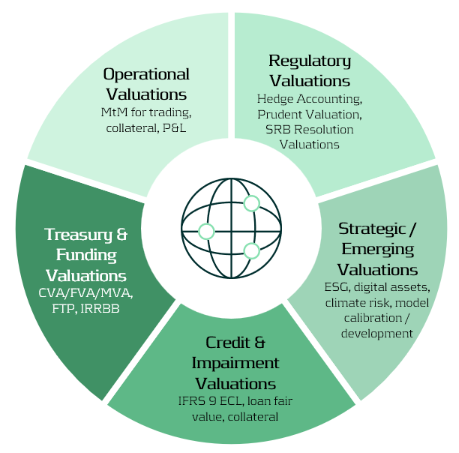
Valuation lies at the heart of financial institutions — informing decisions in trading, risk management, collateral management, accounting, and financial reporting. Yet across many banks, these valuations are performed in fragmented silos for different purposes, using different models, data sources, and systems. In addition to these core applications, valuations also support a broader range of activities, including treasury, regulatory reporting, and emerging domains such as ESG and digital assets.  

As illustrated in the Valuation Map (Figure 1), we observe that in many cases different departments conduct their own valuations, often for their own distinct purposes and using distinct valuation processes. Survey evidence shows that finance and FP&A teams devote roughly 65% of their time to data gathering, cleaning, and reconciliation, leaving only about 35% for value-adding analysis¹.

The Cost of Fragmentation 

Fragmented valuation architectures translate directly into higher costs and operational drag. In practice, three effects are most pronounced: 

• High data vendor spend –  market-data pricing surveys found that some firms were paying “many multiples” more than peers for similar products and use cases, reflecting redundant sourcing and poor usage visibility².

• Model proliferation – large banks often operate with hundreds to thousands of models across the enterprise, creating overlap in purpose and increasing governance, maintenance, and compute costs³. 

• Inconsistent and time-consuming valuations – disparate models and data feeds lead to unclear ownership of valuation “truth” and significant manual reconciliation between accounting, risk, and front-office views. 

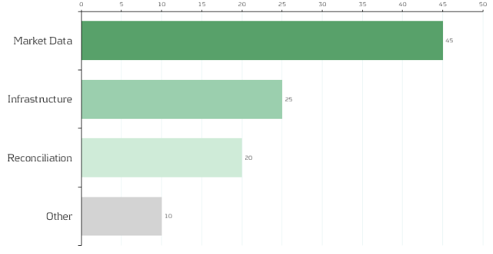
Although no public benchmark precisely mirrors our allocation, multiple industry surveys converge on the same conclusion: market data represents a dominant share of valuation costs, and fragmented reconciliation processes account for a significant portion of non-value-adding effort. Figure 2 therefore shows an indicative distribution — 45% market data, 25% infrastructure, 20% reconciliation, 10% other — to convey the relative scale of each component. Institutions will vary in mix, yet the implication is consistent: rationalizing data sourcing and automating reconciliation are among the highest-impact levers for reducing total valuation cost. 

Strategic Imperative: Centralizing and Standardizing Valuation 

Banks can unlock substantial efficiency gains by centralizing valuation logic and governing data flows. Similar to how treasury departments manage liquidity, banks should treat valuation processes as coordinated enterprise capabilities rather than fragmented operational activities.  

Key levers include: 

1-Valuation as a Service (VaaS): 

Establish a centralized valuation engine providing consistent pricing APIs for all functions (risk, finance, collateral, etc.). 

2-Unified Market Data Platform: 

Integrate vendor feeds into a single validated golden source with standardized identifiers and governance. 

3-Model Consolidation and Validation: 

Maintain one approved model per product type with clear ownership and lifecycle management. 

4- Process Automation: 

Automate reconciliation between accounting and risk views via shared data lineage and valuation transparency. 

5- Cost Transparency: 

Track valuation and data usage per business unit to encourage accountability and optimization. 

Together, these measures reduce duplication, accelerate reporting cycles, and improve consistency across valuation outcomes. 

Building the Foundation 

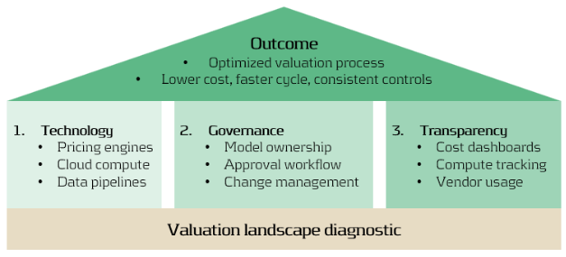
An optimized valuation operating model rests on three mutually reinforcing foundations:  

• Technology: Scalable pricing engines, cloud compute elasticity, and efficient data pipelines. 

• Governance: Clear model ownership, approval, and change management across risk and finance. 

• Transparency: Dashboards tracking valuation cost, compute time, and data provider usage. 

A practical first step: Zanders can perform a valuation landscape diagnostic, mapping all valuation types, systems, and data sources. Such analysis typically reveals 10–20% potential overlap and quick wins in data consolidation⁴. 

Conclusion: Elevating Valuation Processes to an Enterprise Capability 

In today’s environment of cost pressure and regulatory scrutiny, optimizing valuation processes is not only about efficiency—it is about strengthening consistency, transparency, and trust across the organization. Institutions that unify valuation workflows, data, and governance are better positioned to: 

• Reduce operational costs and reconciliation workloads. 

• Rationalize compute power – costs of running multiple models unnecessarily. 

• Strengthen governance and auditability. 

• Accelerate model deployment and reporting cycles. 

• Enable transparent, sustainable, and data-driven decision-making. 

At Zanders, we design and implement integrated valuation frameworks at leading financial institutions, that combine operational efficiency with regulatory robustness. 

If your organization is looking to streamline valuation processes, harmonize market data, or reduce reconciliation workloads, we invite you to connect with our experts.

As part of our ongoing series on the ECB’s 2026 Geopolitical Reverse Stress Test, we previously explored why channels matter more than numbers and how geopolitical risk shapes failure pathways in reverse stress testing.

Why This Matters

A key objective of the ECB’s 2026 Reverse Stress Test is for banks to assess the resilience of their business model. This requires a comprehensive taxonomy of geopolitical risk drivers linked to business impact via plausible transmission channels. Without this foundation, reverse stress testing becomes guesswork, blind to hidden vulnerabilities and hard to defend under supervisory scrutiny.

Step 1: Identify and Engage the Right Stakeholders

Creating a useful taxonomy is not a siloed exercise. It requires bringing together a cross-functional working group: risk management to define categories and metrics, treasury and finance to assess balance sheet sensitivities, business lines to validate exposures, geography and concentrations, compliance and legal to capture sanction regimes and regulatory constraints. Early engagement ensures the taxonomy reflects the bank’s unique business model and risk profile.

Step 2: Structure the Taxonomy Using a Layered Approach

The starting point is to move from broad geopolitical themes to tangible impacts. Begin by identifying high-level drivers such as sanctions, trade fragmentation, energy disruption or military escalation.

From there, think about how these drivers ripple through the organization—through financial markets, the real economy, and safety & security. The goal is to connect these channels to your business model and balance sheet exposures, and then drill down to measurable risk parameters like PD/LGD shocks or market sensitivities.

Step 3: Apply Robust Modelling Approaches and “Reverse-Orientation”

Once the taxonomy is defined, the next step is to make it actionable. Start with scenario-based analysis to explore plausible geopolitical shocks and their effects across channels. Then, use sensitivity screening to identify which sectors and counterparties are most exposed.

It is not uncommon for this exercise to yield a constellation of viable assumptions leading to the desired outcome; quantitative methods, such as Monte Carlo simulations or optimization methods, can aid in exploring the solution space and guide in the choice of the scenario which best fits the profile and narrative of your organization. The aim is not to build the most complex model but to ensure the taxonomy translates into meaningful insights for decision-making.

Step 4: Leverage External Data and Benchmarks

No taxonomy should be built in isolation. External data adds credibility and depth. Regulatory guidance from the ECB provides a clear baseline, while industry benchmarks and rating agency data can help calibrate sector sensitivities.

Geopolitical risk indices and historical stress events offer valuable context for scenario design. Combining internal insights with external references ensures your taxonomy reflects both supervisory expectations and real-world dynamics.

Step 5: Establish Governance and Documentation

Finally, governance is what turns a taxonomy into a trusted framework. This means securing board-level oversight, involving cross-functional committees, and maintaining clear documentation of assumptions and methodologies.

Regular updates are essential, as geopolitical risks evolve. A well-governed process not only satisfies regulatory scrutiny but also embeds the taxonomy into the bank’s risk culture, making it a living tool rather than a one-off exercise.

How Zanders Can Help

We guide banks through this process end-to-end:

• Quantitative modeling to support or benchmark scenario design.
• Advisory support to design and validate a complete taxonomy.
• Hands-on assistance during stress test exercises, leveraging experience with European banks.
• Tooling development or deployment of our Credit Risk Suite (CRS) for scenario modeling, automated ECL/CET1 impact calculations, and advanced optimization techniques.

Transform compliance into strategic capability for resilience. Contact us to find out how we can help your organization.

Read our previous blog on ECB 2026 Geopolitical Reverse Stress Test.

Why This Matters

For banks, the ECB’s 2026 thematic reverse stress test on geopolitical risk is more than a regulatory exercise. It’s a reality check on failure pathways. The cost of missing how shocks transmit through your business can be severe: capital depletion, liquidity strain, and reputational damage when the next crisis hits.

This is not about ticking boxes or plugging in generic macro scenarios. It is about demonstrating to supervisors and to your board that you understand which channels could break your business model and how those channels map to tangible impacts on capital, liquidity, and operations.

In reverse stress testing, you start from a pre-defined failure outcome and work backwards to plausible scenarios that could cause it. In our previous blog, we argued for a bank-specific taxonomy of geopolitical risk drivers because reverse stress testing is only credible when the transmission channels are correctly selected and explained. Today, we take the next step: translating a risk driver into business‑model impact that can credibly produce the failure condition.

Worked Example: Military Escalation

In the context of Military Escalation, as an illustrative example, let’s consider a conflict disrupting shipping lanes in the South China Sea. The chain of transmission may unfold as follows:

• The incident would disrupt global trade routes, creating severe supply chain¹ bottlenecks and driving up costs for  industries depending on imports from and exports to the region. These disruptions would ripple through the real economy, affecting manufacturing, logistics, energy and semiconductor² sectors, and ultimately impacting banks with concentrated exposures in these sectors.

• Investors would seek safe assets, triggering sharp movements in commodity and foreign exchange markets. Banks with open positions in these markets could face significant mark-to-market losses, while liquidity strains emerge as funding costs rise. In addition, cargo insurance premiums on conflict‑adjacent corridors can spike, prompting re-routing and a broader repricing of risk.

• Operational risks would likely increase. Military tensions often coincide with heightened cyber and/or physical threats, increasing the likelihood of state-sponsored attacks on financial infrastructure. Banks would need to increase investment in cyber defence and resilience measures.

• Sanctions may be imposed by multiple parties, exposing banks to potential breaches and contractual disputes with counterparties linked to conflict zones. This adds complexity to transaction screening and legal oversight.

• Finally, these channels translate into measurable risk parameters. Credit portfolios tied to vulnerable sectors would see severe PD shocks, alongside LGD adjustments for collateral impacted by trade restrictions. Together with the market and operational risk impacts described above, they could erode CET1 ratios, revealing failure pathways that standard stress tests might miss.

Reverse The Logic

Because a reverse stress test starts from the outcome, the final step is iterative - the engine room of the exercise. To reach the targeted impact (300 bps CET1 depletion in the ECB’s thematic exercise), you will likely cycle through the channel, mechanism, risk‑parameter mapping and tune the shocks, strengthening or weakening their severity and duration until the constellation of assumptions consistently delivers the failure condition. But a key fallacy is to treat this as a mechanic “tuning” exercise rather than a careful consideration of which combination of shocks and channels that plausibly will drive CET1 below the threshold?

Scaling This Approach

The method extends to other relevant drivers: sanctions, energy disruptions, cyber threats, but the taxonomy must be granular and defensible, with a clear line‑of‑sight from event to channel, and then to portfolio, risk parameters and capital metrics. This strengthens Reverse Stress Testing credibility and ICAAP alignment, and produces governance‑ready narratives for senior decision‑makers.

How We Can Help

We support banks in building a robust RST framework. Our approach includes:

• Advisory support to design a purposeful, bank-specific taxonomy and link it to ICAAP.
• Quantitative modeling to support or benchmark scenario design.
• Hands-on assistance during stress test exercises, leveraging our experience with several European banks.
• Tool development and deployment of our Credit Risk Suite (CRS) for scenario modeling, automated ECL and CET1 impact calculations, and advanced scenario building.

With Zanders, you can move beyond compliance to create a stress test framework that enhances your strategic capability.

Introduction: Why This Matters Now 

Geopolitical risk has become a defining feature of today’s financial landscape. Trade fragmentation, sanctions, and regional conflicts are reshaping markets and business models. Recognizing this, the European Central Bank (ECB) will run a thematic Reverse Stress Test (RST) on geopolitical risk in 2026 as part of its explicit supervisory priorities. Unlike traditional stress tests, RST starts from a failure condition and works backward to identify plausible scenarios that could lead to this situation.  

Hence, this exercise is not about plugging in generic macro shocks—it’s about uncovering hidden vulnerabilities. And that requires one critical ingredient: an informed and detailed view of how geopolitical events may affect your organization. 

The Key Challenge: Seeing the Full Picture 

To pass muster with supervisors, selecting and explaining the transmission channels will matter far more than the numerical modeling. If relevant channels are missed, the backward search becomes blind, undermining the credibility of the entire exercise. The ECB has made clear that banks must go beyond traditional macroeconomic modeling and identify how disruption to trade flows and supply chains, cyberattacks, and even physical risks related to conflicts might affect banks and their clients, and in turn how this transmits to banks’ capital, liquidity, and operations.  

While the ECB has mapped out the primary pathways through which geopolitical risks propagate, the size and nature of the impact will very much depend on each bank’s location, exposures, and business models — meaning a one-size-fits-all approach will not work. Reverse stress testing is designed to uncover failure pathways, but this only happens if transmission channels have been studied and selected with care.  

Building a granular, bank-specific taxonomy of geopolitical risk drivers and their linkages to the portfolio is therefore a critical step. 

What Does a Geopolitical Risk Taxonomy Look Like? 

Well-defined transmission channels should link high-level risk drivers to specific impacts and risk parameters. For example: 

• Drivers: Trade tensions, sanctions, regional conflicts, cyber threats, energy disruptions, and overall market volatility. 

• Impacts: Credit losses (through direct and indirect exposures), loss of revenue (loss of markets, loss of pricing power), cost increases (funding costs, safety and security measures, insurance premiums, staff compensation and relocation), compliance and legal risks (sanctions breaches, disputes). 

• Risk Parameters: PD and LGD shocks, market risk factors, operational risk metrics. 

Once relevant transmission channels have been defined and quantified, the severity of the shocks to the risk drivers can be tuned so that the targeted reverse stress impact is achieved. In the case of the ECB reverse stress test, a CET1 capital impact of 300 basis points is targeted. Finding a balanced set of shocks to achieve the reverse stress target will require expert judgement and needs to be documented properly. 

A layered approach like this will help ensure that the exercise does not become a paper product but a strategic diagnostic tool that meets supervisors’ expectations. In our next blog, we will spend more time on how to set up a proper taxonomy and make it actionable for your organization. 

How Zanders Can Help 

At Zanders, we support banks in building a robust RST framework. Our approach includes: 

• Quantitative modeling to support or benchmark scenario design.  

• Advisory support to design a purposeful, bank-specific taxonomy and link it to ICAAP. 

• Hands-on assistance during stress test exercises, leveraging our experience with several European banks. 

• Tool development and deployment of our Credit Risk Suite (CRS) for scenario modeling, automated ECL and CET1 impact calculations, and advanced scenario building. 

With Zanders, you can move beyond compliance to create a stress test framework that enhances your strategic capability.

Over the past decade, regulatory expectations on European banks’ ESG frameworks have evolved from voluntary disclosure initiatives to detailed operational requirements. While certain regulations such as CSRD and CSDDD have been watered down as part of the Omnibus Directive, EUs climate goals and Climate Law remain intact. The EBA Guidelines on the management of ESG risks will come into force in January 2026, mandating all but the smallest banks to submit annual plans demonstrating how they will reduce their portfolio emissions in time to meet internal and external targets.

Ironically, amidst a slower-than-expected decarbonization in society in general, and with several American and international banks retreating from their climate commitments (and the ensuing collapse of the Net Zero Banking Alliance), it is European banks that are exposed to the largest compliance and reputational risks.

In our experience, many banks may have underestimated the far-reaching impact of the new Guidelines. Unlike previous regulatory guidance, including ECBs Guide on climate-related and environmental risks, what is now required is the complete integration of ESG risks and targets into banks’ ways of working: risk management, client engagement, operations, pricing, and business strategy.

Below we outline the four areas we think will prove the most challenging for banks to implement.

Key challenges

1. Data availability and processes

Banks are required to have in place a structured data environment to enable assessment of ESG risks, with the explicitly stated aim that most of the data should be sourced at the client- and asset level. The Guidelines list a number of metrics that large institutions must define and monitor, including:

• Financed emissions (Scope 1-3)
• Portfolio metrics of clients that are, or are projected to be, misaligned with emission targets
• A breakdown of portfolios secured by real estate according to the level of energy efficiency
• Metrics related to dependencies and impacts on ecosystem services, in particular water
• Metrics related to ESG-related reputational and legal risks (via the banks’ exposures)

Some of these data are already collected and reported by banks, such as financed emissions. But even those metrics rely largely on proxies and assumptions. Even among PCAF member banks the variation in reported emission intensities is significant - and in many cases inexplicable. For many other metrics the data to construct them is either missing or has not even been defined.

Banks need to accelerate their ESG data strategy and decide, for the short- and medium, which data to collect directly from clients andwhich to source from external providers, and the data gaps for which there are no viable alternatives but to use proxies. In turn, for each of these categories there will be many choices to make with implications for quality, timeliness, and costs. In parallel, but informed by the data strategy, the bank needs to decide on – and invest in - their future data infrastructure, which may take years to realize. One obvious case is the need to connect real estate characteristics, such as LTV, flood exposure, energy rating, and insurance coverage with clients’ financial data as well as outputs from climate scenario models.

2. Models and Methods

The Guidelines require banks to map ESG risk drivers to traditional risk categories and – if they are material - embed the risks in several processes: collateral valuation, ICAAP, stress testing, underwriting, and pricing.

The first step in this exercise is to determine which risk drivers are material, and for which risk types. In the end, for most banks, physical and transition risks stemming from climate change will likely prove the most material for credit risk, but ECBs expectations as to the rigor of the materiality assessment - to substantiate such a conclusion - are increasing. For example, banks need to have methodologies in place to assess how and whether social and governance failures in client firms may result in both financial as well as reputational and legal risks.

Even for key risk drivers such as flood risk, banks face a significant challenge in quantifying how and with which probability this will translate into credit risk. It necessitates a number of assumptions such as the response in real estate prices and insurance costs/availability, as well as government policy and disaster funds, flood protection work, and much more. Limited or absent historical data together with the changing nature of risks related to climate change make this kind of model development very different from traditional risk modeling in banks (such as IRB model) and necessitates new expertise.

And while there are several useful publicly available models, in particular by the Net Greening of the Financial System, there is still a lot of work to be done to adapt those scenarios to individual banks’ portfolios and business models.

3. Client engagement and risk assessment

EBA expects climate and environmental risks to be factored into client selection, due diligence, covenants and pricing based, for a start, on an evaluation of counterparties’ transition readiness and resilience to physical risks. Even for large clients that are reporting under CSRD, a lot of the data required to perform these assessments will have to be collected directly as part of the onboarding process.

Although many banks have separate ESG advisory units that support client executives, these are often there to identify opportunities for sustainable products and loans and are not trained to assess and quantify clients’ risks. In the end, it is client executives and credit committees that must stand over the ESG risk assessment and its impact on credit scores, pricing and loan conditions. To save costs and time for client-facing staff, they should be equipped with practical and user-friendly tools and systems that support them in collecting and organizing relevant ESG data.

Worse, for most SME and retail customers there is no dedicated account manager, the on-boarding and credit process is largely automated. Banks should develop a risk-based sourcing strategy that, at least initially, uses sector-level proxies for the majority of firms while collecting individual data from those that have been designated as high-risk clients. Again, a number of choices have to be made when developing such a framework to ensure it is purposeful.

4. Governance and steering

What we deem most pressing  for banks is to decide on their governance to triage and drive progress on the vast array of requirements. It will require strong leadership and a project committee with sufficient seniority to make crucial, and potentially costly decisions. Elaborate RACIs will be of little use if those assigned ownership are found too low in the bank’s hierarchy.

While the exact division of responsibilities will depend on each bank’s structure and governance model, it is clear that the actual transition plan(s) should be owned by the first line (and subsequently validated by second line), and tie into existing business planning and strategic process.  At the same time, the transition plan will be part of the annual ICAAP submission, which is a second-line responsibility, and the bank’s ESG strategy should be reflected in the business resilience test . Hence, these first- and second-line processes must be aligned.

The Board and CEO should set the bank’s ESG strategy and ensure that these expectations are actionable. Little progress is to be expected if C-suite members do not have clear KPIs and KRIs tied to the delivery of the bank’s transition plan. Quantitative targets may be based on, in addition to financed emissions, the energy efficiency profile of the mortgage book, sustainability-linked bond issuance, and the funding of low-carbon power production. Such targets may necessitate difficult trade-offs, including tighter origination criteria, off-boarding of high-risk clients, and larger discounts for green loans.

Purposeful implementation strategy

To succeed in this potentially daunting endeavour banks should adopt a pragmatic implementation approach, balancing costs against compliance risks. The ECB and local supervisors are fully aware that banks need considerable time to get all prerequisites in place, and the scope and detail of transition plans must be allowed to evolve over years.

However, while early transition plans cannot be expected to present the ultimate answers to either data, methodological or governance challenges, , banks should be able to demonstrate their capacity to achieve essential climate and environmental objectives. Quantitative targets, in particular regarding a bank’s financed emissions, must be achievable.

Finally, underscored by recent legal cases, any claims related to the bank’s “green” credentials must be based on evidence. The heightened compliance and legal risks mean that it is timely to review the bank’s public as well as non-public ESG commitments, benchmark them against peers, and make an honest assessment of the costs and resources necessary to fulfil them.

Want to find out more about how Zanders can assist your bank in developing your ESG strategy and meet regulatory expectations?

Reach out to our Partner Lars Frisell, our ESG and risk management expert, for tailored guidance.

For treasury and finance teams, this isn’t merely an accounting tweak. It changes how liabilities, assets, and liquidity are presented at reporting cut-offs, with considerable implications for system configuration and investor perception.

What has changed?

Under past practice, liabilities typically were removed from the balance sheet as soon as payment instructions were sent to a bank. Under the updated standard, such derecognition is no longer permitted unless settlement has actually occurred and funds are in the hands of the counterparty.

This change aligns accounting more faithfully with economic reality: until settlement occurs, the liability remains and cannot be considered discharged.

In SAP, liabilities are often cleared at the payment run step, with postings to a cash-in-transit (“CIT”) account.

Example: SAP F110 + CIT vs Settlement-Date

Steps	Old Practice (Instruction Date / CIT)	New Requirement (Settlement Date)
31 Dec, Payment run executed in SAP F110	Dr AP CR CIT (Liability Cleared, cash-in-transit posted)	Liability remains in AP no derecognition yet
1–2 Jan, Funds in transit supplier not yet paid	Liability already derecognised; balance sits in CIT (classified as cash)	Liability still shown as outstanding in AP
2 Jan, Bank statement import confirms settlement	Dr CIT CR Bank	DR AP CR Bank Liability cleared at settlement

Impact: Under the old method, liabilities disappeared prematurely and cash was overstated, creating distorted liquidity positions. Under IFRS 9, derecognition only happens when settlement is confirmed by the bank.

The same timing challenge applies in in-house bank (IHB) scenarios, where intercompany positions are often cleared in SAP before external settlement has actually taken place.

This change aligns accounting more faithfully with economic reality: until settlement occurs, the liability remains and cannot be considered discharged.

Why the IASB stepped in

The previous method often led to distorted liquidity positions. Liquidity, as shown on the face of the financials, could appear stronger than warranted while liabilities looked lower. The IASB’s concern lay in classification, timing, and how external users interpret financial statements.

The effect can be seen in the example below:

Approach	Current Assets	Current Liabilities	Current Ratio
Settlement-date accounting	€100,000	€10,500	9.5
Instruction-date accounting	€90,000	€500	180.0

In the table above, we can see that the economic position under both approaches remains identical, the supplier is unpaid and the cash is still in the bank. The difference lies in the presentation. Under instruction-date accounting, liabilities appear lower, making liquidity look stronger than it truly is. Under settlement-date accounting, liabilities remain on the balance sheet until cash is received by the counterparty. This provides a more faithful representation of the company’s financial position and addresses the IASB’s concern that inconsistent reporting reduces comparability and distorts how investors perceive liquidity and risk.

The Exemption

For financial liabilities only, IFRS 9 allows an optional policy election, companies may derecognise at the instruction date but only for payment systems (e.g. CHAPS or SEPA) that meet stringent criteria. Derecognition at instruction date is permitted only if:

• the payment instruction is irrevocable
• the entity cannot access or redirect the cash after initiation
• settlement risk is insignificant
• settlement is expected to occur within a very short timeframe

If this exemption is elected, it must be applied consistently within that payment system. Companies can choose different approaches for different systems for example, applying the exemption to SEPA but not to CHAPS.

While this option can provide operational relief and reduce the need for immediate system changes, it may also increase configuration complexity where multiple payment systems are used.

For example in SAP this choice needs to be reflected in payment method configuration, house bank integration, and clearing logic. While the exemption may reduce the need for immediate system changes, it can add a high level of complexity where multiple payment systems are used. The exemption also requires clear disclosure under IFRS 7.

What companies should do now

The degree of impact will vary. Entities with high volumes of electronic payments, in-house bank models, or complex treasury workflows are likely to be most affected.

For SAP users, the priority is to map where liabilities are currently being derecognised before settlement and focus on updating configuration in the following key system areas:

• Payment run (F110): Review clearing logic and postings to CIT. Ensure liabilities remain in AP until the bank statement import (EBS) confirms settlement.
• Bank statement processing (EBS): Confirm settlement recognition logic, including how postings flow from house banks to AP and cash accounts.
• Cash and liquidity reporting (Fiori apps): Validate whether Cash Position and Liquidity Forecast details reflect settlement date logic and align with IFRS 9 reporting.
• Payment method & House Bank configuration: If the IFRS 9 exemption is applied, ensure configuration is consistent at the payment system level, and correctly applied to exemptions only.
• Accounting configuration: Review and update how cash-in-transit (CIT) postings are set up in SAP.

Aligning SAP configuration across these areas is essential to ensure management reporting and statutory reporting remain consistent and to avoid distorted liquidity views at reporting cut-offs.

For many companies, these changes are not just a simple adjustment to accounting treatment they will require extensive configuration updates across SAP treasury and banking processes. Delaying the review could leave year-end reporting out of step with IFRS 9.

How we can help

These amendments reshape how liquidity and financial strength are communicated to stakeholders. With the effective date approaching, companies should act pre-emptively: assess exposure, evaluate options, and prepare systems and processes for change. Our team combines IFRS expertise with deep SAP treasury and technology knowledge, helping organizations translate regulatory change into practical implementation. To explore how the IFRS 9 amendments may affect your reporting, SAP configuration, or liquidity metrics, please get in touch with our advisory team, Jordan James, or Deepak Aggarwal.

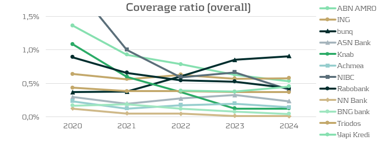
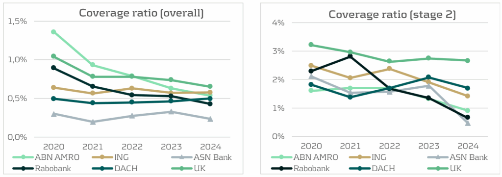
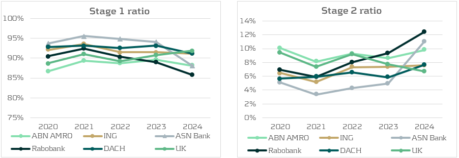
This article first analyzes trends in coverage ratios among 13 Dutch banks¹, and puts the results of the largest Dutch banks in international context. Furthermore, this article builds on previous annual studies (2023 and 2024). For this purpose, coverage ratios and stage exposures from the four largest Dutch banks are compared with the five largest UK² and DACH³ banks as benchmarks. Next, macroeconomic outlooks from a group of Dutch banks are discussed. Finally, the application of management overlays by all Dutch banks is discussed as well.

In general, the results show continuation of a decreasing trend in the coverage ratio for Dutch banks, which is a persistent trend since 2020. From a bank’s perspective, this is a positive development: lower coverage ratios are driven by improved macroeconomic conditions, reduced manual overlays and healthier portfolios, and therefore leading to lower Expected Credit Losses (ECL). Especially Stage 2 coverage ratios are lower in 2024, as changes in macroeconomic outlooks have a stronger effect on these loans because ECL for Stage 2 are determined over the lifetime of the loans. The transfer of loans from Stage 1 to Stage 2 also happened persistently over the last couple of years. This could be seen together with the EBA monitoring report (IFRS 9 implementation by EU institutions) which called for a more conservative and broader definition of Stage 2. The increase in Stage 2 ratios is a counterintuitive finding when paired with the decrease in coverage ratios. As Stage 2 reflects a Significant Increase in Credit Risk (SICR), credit loss provisions are expected to be higher. However, it follows that the effects driving the coverage ratios down outweigh the increase in Stage 2 exposure.

Coverage Ratios: a Decreasing Trend

The Dutch banks are expecting lower credit losses compared to previous years, resulting in lower coverage ratios. There are three main drivers for this. Firstly, several banks (e.g. ASN Bank) mention a significantly more positive macroeconomic outlook. The second driver is not forward-looking but is a realization of higher-than-expected increases in house prices in 2024. As mentioned by ABN Amro and Rabobank, the Dutch house price index (HPI) was expected to rise around 2% in 2024, while this turned out to be 9%. Higher house prices improve collateral values and therefore lower the future Loss Given Default (LGD) in case of a mortgage default in the IFRS 9 models. The third driver behind lower ECL is that many banks decreased the management overlays to the model outcomes in 2024 compared to 2023. Combining these three drivers pushes coverage ratios down.

In international context, the largest Dutch banks are well positioned compared to banks in the UK and DACH regions. The coverage ratio of UK banks is relatively high but is decreasing due to improvements in economic outlooks and a decrease in inflation. The coverage ratios of DACH banks are comparable to those of the Dutch banks. However, the coverage ratio of the DACH banks did increase slightly compared to 2023, driven by a weak German economy and the increased geopolitical risk of US trading wars. Although the expectation of a trading war has worldwide implications, there are several reasons why the German economy would suffer more from this than the Dutch or English economies. Firstly, Germany is the most reliant on export out of these three countries, with over 50% of its GDP allocated to exports. Secondly, German banks lend heavily to autos, machinery, and chemicals, exactly the industries most exposed to US tarrifs. In contrast, Dutch banks rely more on agriculture, mortgages and domestic real estate. UK banks are more globally diversified, giving them a smaller exposure to US trade wars. For these reasons, the effect of potential US trade wars is weighed more heavily into the macroeconomic IFRS 9 scenarios for German banks.

Stage Ratios: Counterintuitive Movements

Another development in 2024 is the increase in Stage 2 exposures at Dutch banks. Rabobank, ASN Bank, and ABN Amro all reported more Stage 2 loans, largely the result of framework updates and stricter Significant Increase in Credit Risk (SICR) definitions. At Rabobank, an ECB regulation and Risk Based Strategy approach was implemented in the Stage 2 framework for residential mortgages, raising the allowances for ECL. The increase is predominantly related to mortgage clients who have not voluntarily provided updated financial income information. Hence, the increase in Stage 2 ratio is not caused by an increase in the risk of default but because the framework required a risk-based treatment of missing data. Combined with a decrease in Stage 1 exposures, it is concluded that these loans transferred from Stage 1 to Stage 2. ASN Bank also confirms this trend by a large transfer of interest-only mortgages from Stage 1 to Stage 2.

Even though more loans are classified as having a SICR, there is no negative impact on coverage ratios. The overall coverage ratios decrease and the Stage 2 coverage ratios decrease sharply. When macroeconomic outlooks improve, this has a significantly larger impact on Stage 2 coverage ratios than on Stage 1 coverages due to the lifetime ECL estimation of Stage 2 loans. The more conservative design of the Stage 2 framework has been noted by the ECB, who reported an increase in the share of Stage 2 loans without a significant increase in default rates (Same but different: credit risk provisioning under IFRS 9). This trend is empowered by the EBA, who encouraged banks in their previously mentioned report to be more conservative and shift more assets to Stage 2.

Outside of the Netherlands, the trend of increasing Stage 2 exposures at the expense of Stage 1 is also visible in the DACH region, where for the five largest banks the Stage 2 ratio increased from 6% to 8%. This increase is also paired with a decrease in the Stage 2 coverage ratio. Conversely, the UK banks do not show this trend and even report decreasing Stage 2 ratios paired with increasing Stage 1 ratios. As the UK banks do not fall under ECB supervision or EBA authority, they are not subject to the same trends observed for EU banks.

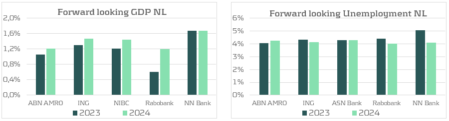
Improved macroeconomic outlooks

For the analysis of macroeconomic outlooks, the focus is on the Dutch banks as these outlooks are often for the national economy and thus not comparable between countries. In practice, most Dutch banks define three scenarios (base, up, down) and the average allocation is 50% to the base scenario, with the remaining 50% skewed to the downside (32%) rather than the upside (18%). Although the probabilities have not been skewed positively, the outlook of all scenarios has improved compared to 2023. The five Dutch banks reporting their forward looking GDP figures all show improvements, with only NN Bank holding the prediction from last year. At the same time, the predicted unemployment has decreased for most banks reporting this figure. Both of these signal the improved macroeconomic conditions that lead to lower ECL.

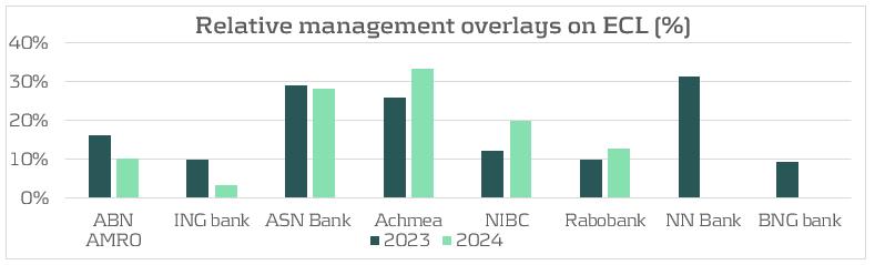
Reduction in Management Overlays

The second driver behind the lower coverage ratios is the decrease in management overlays, which most banks reduced in 2024 compared to 2023. Overlays remain an important tool to capture risks not covered by the models, as also highlighted by the ECB in 2024 (IFRS 9 overlays and model improvements for novel risks). While the ECB welcomes the use of overlays to capture novel risks, it also warns for misuse. Specifically, the ECB would like to see overlays applied at the parameter level, and not at the total ECL level, as most Dutch banks do. According to the report there is still room for a lot of improvements in the use of overlays in IFRS 9 modeling. Amongst the Dutch banks, the average overlay decreased from 11% in 2023 to 8% in 2024. ABN Amro discontinued the overlay for geopolitical risk and decreased the overlay for nitrogen reducing measures on livestock farming business. ING decided to fully abandon the management overlays in place for the Covid-19 support program, which had been in place for several years. Other overlays like those for climate transition risk, mortgage portfolio adjustments and inflation and interest rate increases were reduced but are still in place. Some other banks, like BNG and NN Bank completely discontinued all management overlays. For NN Bank, the previous overlay was in place related to rising interest rates and high inflation. As for BNG, the overlay was meant to account for an increased risk for the healthcare sector. After a thorough evaluation of the sector, BNG has concluded that the models now correctly reflect the risks in the healthcare sector and the overlay is no longer required.

Most management overlays are applied to cover macroeconomic risks, such as interest rate risk, inflation risk and geopolitical risk. After the EBA concluded in the previously mentioned report that climate and environmental risks were covered insufficiently, some banks have also started applying more overlays regarding this area. Other banks, like BNG, have started improving the modeling to account for climate-related matters in ECL calculations. These model improvements have not been completed yet. Additionally, some banks do recognize and investigate climate and environmental (C&E) risks but do not quantify these risks in their IFRS 9 frameworks, such as NN Bank.

What can Zanders offer?

The results from the annual report study of 2024 show that approaches and results between banks for the IFRS 9 framework still differ greatly and there remain many modeling improvements to be made. These differences do not stem from the model itself, but rather from how models are applied. Key drivers include the composition of loan portfolios, the SICR frameworks, and the design and weighing of macroeconomic scenarios. It is worthwhile to investigate how Dutch banks can learn from each other in modeling ECL. For any bank, it is useful to assess their current IFRS 9 framework and critically evaluate whether it is line with the actual expectations on future credit losses.

As Zanders has a focus on the Dutch market but also has a presence in the UK and DACH regions, we are in constant contact with many of the active banks in these regions. This makes us the best strategic partner to help you with improving your IFRS 9 modeling.

If you need help with your IFRS 9 models or want to learn more about these IFRS 9 results to see how your results fit in, please contact Kasper Wijshoff.

Building on the June 2024 launch of the new EU AML/CFT framework and the creation of the Anti-Money Laundering Authority (AMLA), SupTech (short for Supervisory Technology) now stands as a key driver of more efficient, data-driven, and collaborative supervision.

To inform the report, the EBA surveyed national authorities and worked with the European Commission’s AMLA Task Force to identify trends, challenges, and best practices. In this blog post,  we highlight key insights and explore their impact on the financial sector.

Key Insights from the Report

Across the EU, 31 competent authorities reported working on 60 SupTech projects or tools, most of which launched in the last three years. Nearly half are already in production, with others are in development or left as an idea for implementation. The figures below demonstrate the technologies used in SupTech tools, along with the AML/CFT tasks they aim to address.

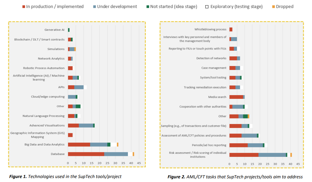
It’s evident from Figure 1 that current efforts focus primarily on improving data quality and scalability, essential foundations for effective SupTech. More advanced technologies like Generative AI, Blockchain, and network analytics are still in early stages but are expected to play a larger role in the future.

On the task side, presented in Figure 2, most tools are geared toward risk assessment, which appears to be the most straightforward application of SupTech. As the technology matures, other areas of AML/CFT supervision may benefit from more advanced capabilities as well.

Advantages and challenges

The EBA’s survey revealed several benefits from current SupTech initiatives, with most projects targeting improvements in data quality, analytics, adaptability, automation, and collaboration through standardization. SupTech enables supervisors to operate more efficiently, respond faster to emerging risks, and make better-informed decisions in a complex financial landscape.

However, fully embracing a data-driven approach comes with challenges. SupTech tools rely heavily on robust IT infrastructure, skilled personnel, and high-quality data. While these tools can help improve data quality by detecting anomalies, they still require reliable input to function effectively.

Legal risks also emerge, particularly around GDPR compliance and accountability for decisions made by opaque algorithmic models. Resistance to adoption may arise due to concerns about job displacement and trust in AI. Additionally, limited collaboration between institutions can lead to duplicated efforts and inefficiencies. Fortunately, the new AML/CFT framework offers a foundation for improved cooperation and information sharing across borders.

How can banks prepare for a successful transition?

Although the EBA’s report is aimed at supervisory authorities, it has important consequences for banks, payment providers, and other obliged entities. SupTech will help supervisors operate more efficiently and gain deeper insights, but it will also raise expectations for the institutions they oversee. Banks should prepare for increased data requirements, more rigorous scrutiny, and pressure to standardize and respond quickly to regulatory changes. While these requirements may pose short-term challenges, they will ultimately support better compliance, risk management, and operational resilience in the long run. In order to get there, Zanders supports institutions in key areas:

1. Increased data demands: AI-driven tools allow supervisors to process and analyze more data, requiring institutions to provide cleaner, more structured datasets.
2. Increased detail orientation: SupTech tools detect anomalies and patterns faster, meaning institutions must ensure accuracy and consistency in their reporting.
3. Standardisation:  EU-wide platforms and data-sharing standards will require institutions to align systems and formats for seamless supervision.
4. Change management: For SupTech to be successfully implemented, organizations must actively build a digital-first culture and encourage staff to move away from existing processes and mindsets.
5. Rapid adaptation: As technology evolves, supervisors will expect institutions to keep pace. Falling behind could lead to compliance gaps.

These challenges require strategic attention and tailored support. 

Are you interested in how Zanders can guide your organization through this transition? Reach out to our Partner Sebastian Marban.

As the European Union increasingly emphasizes robust digital resilience within the financial sector as of January 17^th 2025, the Digital Operational Resilience Act (DORA) has become a critical benchmark for compliance. A recent survey conducted with 23 banks reveals insightful data on their preparedness across various DORA categories. This blog dives into the findings and assess how well banks are positioned in meeting these regulatory standards. 

General Requirements: Solid Foundations, Communication Gaps 

The survey indicates strong compliance with foundational DORA requirements. Almost all banks have designated management functions for digital operational resilience and documented strategies. However, notable gaps exist in communicating these strategies effectively—as highlighted by the sizable number of banks without comprehensive stakeholder communication plans (12 “yes” vs. 11 “no” responses). Additionally, less than half the respondents have formal ICT risk appetite statements approved by senior management, leaving potential gaps in aligning risk management with organizational tolerance levels. 

ICT Risk Management: Comprehensive Yet Evolving 

Banks demonstrate proficiency in risk management frameworks with most having formal processes for risk identification and documentation. However, only about half systematically manage emerging and innovative technology risks—a critical aspect in today's evolving digital landscape. Equally concerning is the relative lack of focus on interconnectedness and concentration risks, with only 12 banks integrating these considerations into their risk assessments. 

ICT Resilience Testing: Gap Between Basic and Advanced Practices 

While regular ICT resilience testing is generally practiced, the adoption of advanced testing methodologies, such as threat-led penetration testing, is limited among the institutes that are required to perform these tests. Variability also exists in the processes for escalating issues and validating results, signifying areas requiring further attention. 

ICT Third-Party Risk Management: Variable Partnerships Management  

The survey reveals that while vigilance exists in maintaining third-party risk management frameworks, there are significant concerns regarding the strength of contractual safeguards and incident management processes. Less than half the banks have robust exit strategies or cater to geopolitical risks—a critical oversight in managing potential external disruptions. 

Incident Reporting: Strong Foundations with Room for Procedural Enhancement 

The incident reporting results indicate well-established bases in documentation and reporting processes. However, training in incident reporting procedures remains less uniform, which could impact consistency in handling real incidents. 

Business Continuity and Disaster Recovery: Recurring Gaps in Comprehensive Coverage 

While the majority of banks report having BCDRPs in place, only 16 ensure comprehensive coverage of all critical business functions. Testing and updating these plans is similarly underwhelming, staying mostly stagnant, which could hinder timely recovery efforts in case of an outage. 

IT-Security: Solid Security Postures with Continuous Improvement Needed 

Encouragingly, all respondents have documented ICT security policies, and most banks have appropriate security controls in place. While programs for regular updates in policies and controls are broadly adhered to, continuous improvement through employee training and periodic evaluations of security measures remains essential. 

Beyond the Checklist: Embedding True Resilience into Operations 

This survey highlights that while the foundations for DORA compliance are well-established within the banking sector, several areas still require strategic enhancements. Bridging communication gaps, enhancing advanced testing, improving third-party engagements, and boosting procedural training will be key to transitioning from foundational compliance to comprehensive resilience. 

These study insights serve to underscore not only the importance of regulatory adherence but also the critical need for continuous evaluation and proactive adaptation of digital resilience strategies amidst ever-evolving digital challenges. As banks continue this journey, the collective focus should remain on creating a more adaptive, secure, and resilient digital future. 

To find out more about DORA compliance and meeting regulatory standards, please contact our partner Martin Ruf.