The DRM Cycle: The Model in Action

The final article from Zanders on the DRM model presents the lifecycle of the DRM model over a single hedge accounting period and the prospective and retrospective assessments that are required to be carried out to ensure that the entity is correctly mitigating its interest rate risk for the assets/liabilities designated for the Current Net Open Risk Position (CNOP). The cycle will be illustrated by Scenario 1C taken from Agenda Paper 4A – May 2023¹. This is a relatively simple example, more complex ones can be found within the staff paper. 

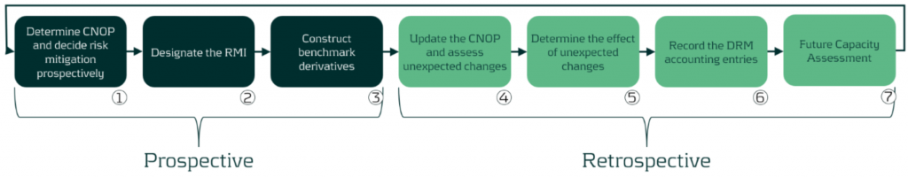
Figure 1: DRM Cycle

Prospective (start of the hedge accounting period)

The first three steps are related to the prospective assessment in the DRM model cycle.  

The use of the prospective assessment is to ensure that the model is being used to mitigate interest rate risk and achieve the target profile that is set out in the RMS. The RMS should include the following: 

• The risk mitigation cannot create new risks 
• The RMI has to transform the CNOP position to a residual risk position that sits within the target profile (TP) 

Step 1: The entity decides on the securities to be hedged and calculates the net open risk position (from an outstanding notional perspective) per time bucket.  

In the example below the company has floating and fixed exposures. The business in this case has a five-year fixed mortgage starting in 20x2 which is fully funded by a five-year floating rate liability. The focus period is 20x2 (start of the hedge accounting period) to 20x3 (end of the hedge accounting period) and so the first period 20x1 has been removed. The entity manages its entity-level interest rate risk for a 5-year time horizon, based on notional exposure in ∆NII and has decided to set the TP to be +/-EUR 500 in each of the repricing periods. Below we present the total fixed and total floating exposures from the product defined above). The individual breakdown of the fixed and floating is not required as each exposure is hedged as a total. The exposure are positions at year end. 

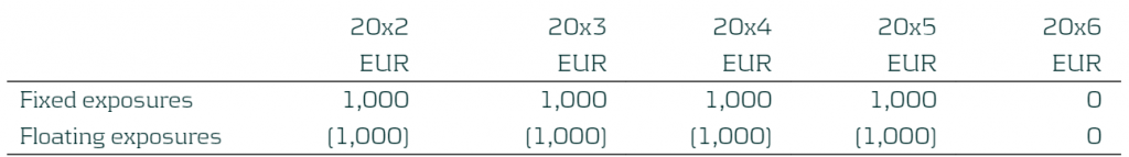
Table 1: CNOP of the Entity with yearly buckets

Step 2: The entity will calculate the RMI based on the designated derivatives. The entity decided to mitigate 80% of the risk through the use of the following derivatives (existing and new). Please note that is a combination of derivatives from all the derivatives available in the books: 

• A 5-year pay fixed receive floating IR swap with notional of EUR 1,000, traded on 1^st January 20x1 (DD Swap 1) (existing deal). 
• A 4-year receive fixed pay floating IR swap with notional of EUR 200, traded on 1^st January 20x2 (DD Swap 2) 

This leads to the designated derivatives with the following exposures: 

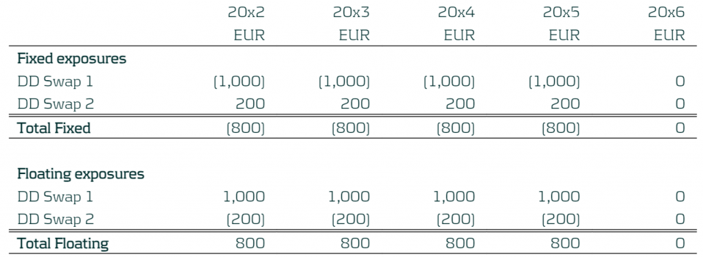
Table: Exposures of the Designated Derivatives 

The exposures of the designated derivatives can then be compared to the CNOP as shown below: 

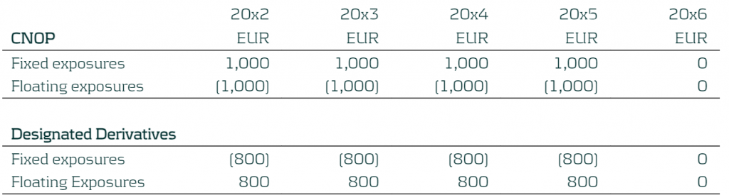
Table 2: Exposures of the CNOP and Designated Derivatives

As the entity manages its interest rate risk based on ∆NII, the RMI focuses on the floating exposure.  

The prospective test is performed by comparing the CNOP and Designated Derivatives exposures at each time bucket to see whether this moves the residual risk inside the TP (+/- EUR 500) set out within the RMS and not providing an over-hedge position. In this case the residual risk will be 0 (80% of CNOP versus DD exposures) and so the prospective assessments pass for all the time buckets. 

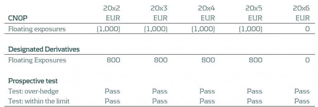
Table 3: Prospective test

Step 3: Benchmark derivatives (hypothetical derivatives) are constructed based on the RMI calculated above.

Table 4: Benchmark Derivatives created for the Fixed and Floating Exposures

Retrospective (end of the hedge accounting period) 

The following steps are related to the retrospective assessment of the DRM model.  

The IASB requires a retrospective assessment, to check that risks have been mitigated, as well as a future capacity assessment for each period². This is to ensure the company is correctly mitigating its interest rate risk, ensuring the CNOP sits within their TP and to quantify the potential misalignment arising from unexpected changes (during the hedge accounting period). 

Step 4: The entity updates the CNOP with the latest ALM information (note that new business is excluded from the updated CNOP). 

In this example, the financial asset was repaid fully at the end of 20x5. The revised expectation is that it will be  partially repaid per end 20x4 and the rest  repaid end 20x5. 

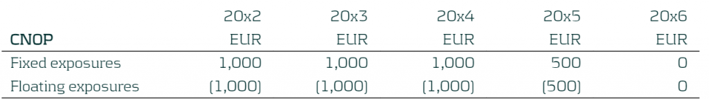
Table 5: Updated CNOP

Step 5: The potential misalignment due to unexpected changes is calculated. The new CNOP is compared to the RMI that was set in Step 2. Misalignments can occur due to: 

• Difference in changes in the fair value of the designated derivatives and  benchmark derivatives (i.e: different fixed rate, fair value adjustments) 
• The effect of the unexpected changes in the current net open position during the period  

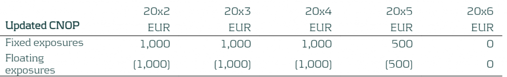
Table 6: Updated CNOP

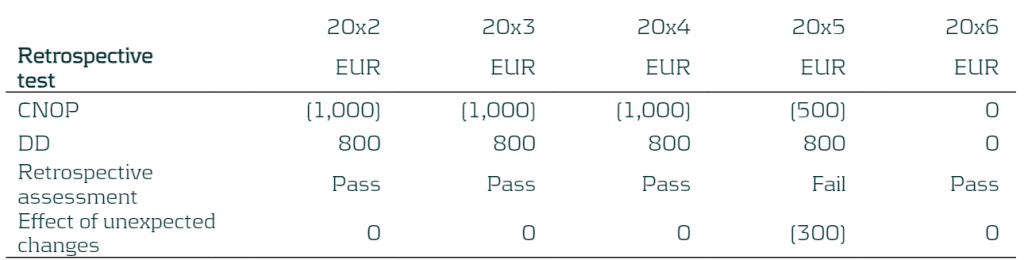
Table 7: Determining the effect of unexpected changes

If there are misalignments and the entity breaches the retrospective assessment, meaning that it has been over-mitigating its risk, the benchmark derivatives will need to be revised. One way in which this can be achieved is through the creation of additional benchmark derivatives which can represent the misalignment occurring. These will be based on the prevailing benchmark interest rates. 

Therefore, for this example, the entity will construct two additional benchmark derivatives to represent these changes: 

• A 4-year pay fixed rate receive floating IR swap with notional of EUR 300, maturing on the 31^st December 20x5 (BD Swap 3) 
• A 3-year receive fixed pay floating IR swap with notional of EUR 300, maturing on 31^st December 20x4 (BD Swap 4) 

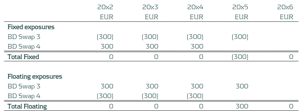
Table 8: Additional Benchmark Derivatives

Step 6: The hedge accounting adjustments are calculated, and the DRM model outputs are required to be booked³: 

• a) The designated derivatives to be measured at fair value in the statement of financial position. 
• b) The DRM adjustments to be recognised in the statement of financial position, as the lower of (in absolute amounts): 
  • The cumulative gain or loss on the designated derivatives from the inception of the DRM model. 
  • The cumulative change in the fair value of the risk mitigation intention attributable to repricing risk from the inception of the DRM model. This would be calculated using the benchmark derivatives (from step 3 and step 5) as a proxy. 
• c) The net gain or loss from the designated derivatives calculated in accordance with (a) and the DRM adjustment calculated in accordance with (b) would be recognised in the statement of profit or loss. 

The table below presents the EUR booking figures for this example. Figures are for the period 20x2 to 20x3. 

The underlying items block represents the interest rate paid/received for the financial asset and financial liability for the period. 

The designated derivative block presents the fair value movement of the designated derivatives for the period and the realised cash flow (net interest rate paid or received) on these instruments (trading income). 

The DRM adjustment block presents the fair value movement of the benchmark derivatives for the period and the realised cash flow on these instruments (trading income). 

BS represents a balance sheet account when IS represents an income statement account.

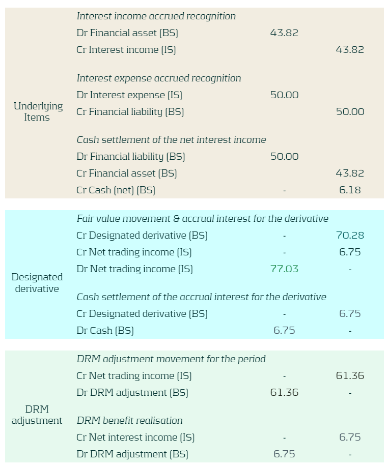
Table 9: Booking figures

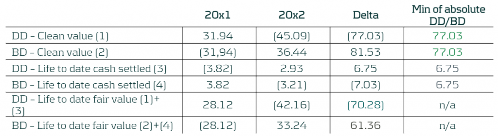
Table 10: Booking figures calculation 

Step 7: The last step is the future capacity assessment which was introduced by the IASB in February 2023 and is still under development so the final implementation of this is still to be released. This step is used to replace the previous retrospective assessment that compared the CNOP sensitivity to the TP. The IASB have yet to release more information on the methodology. The example shown does not assume that the future capacity assessment is carried out. 

What Next?

The IASB plans to publish an exposure draft by 2025 and so companies start thinking about their process for onboarding the DRM model in their accounting process. The DRM model introduces a range of changes to the hedge accounting framework and the transition process will not be an easy switch. Therefore, companies need to ensure that they have a clear and concise implementation plan to ensure a smooth transition. Involvement from stakeholders from across the company such as (IT, Front Office, Risk, Accounting, Treasury) is required to ensure the project is implemented correctly and in time. 

What can Zanders offer?

Transitioning to the new DRM model can be difficult due to the dynamic nature of the model, especially with a more complex balance sheet. Zanders can provide a wide range of expertise to support in the onboarding of the DRM model into your company’s hedging and accounting. We have supported various clients with hedge accounting– including impact analyses, derivative pricing and model validation, and are familiar with the underlying challenges. Zanders can manage the whole project lifecycle from strategizing the implementation, alignment with key stakeholders and then helping design and implement the required models to successfully carry out the hedge accounting at every valuation period. 

For further information, please contact Pierre Wernert, or Alexander Oldroyd.