How do you get banks on board to provide you with financing on favorable terms when your modus operandi isn’t maximizing profit? Zanders helped Royal FloraHolland find the answer, leading them to secure a new debt facility of €210 million with three banks. Royal FloraHolland is the largest B2B floriculture platform in the world. Operating as a member-owned cooperative has always been the strongest element of Royal FloraHolland’s manifesto - right from its first flower auction back in 1912. But this unique structure also proved to be a complication when it came to refinancing its credit facility. Fortunately, they had Zanders on hand to help frame a compelling case for their future credit requirements.

Harnessing cooperative strength

Royal FloraHolland was first established as a cooperative for growers and sellers more than 110 years ago and is renowned for organizing flower auctions via clock sales. Over the years, as the floriculture trade has become increasingly international and competitive, the role and remit of Royal FloraHolland has expanded beyond flower auctions. Today, it is an international B2B trading platform offering a wide variety of deal-making, logistics, and financial services to its members.

Royal FloraHolland - and as a consequence a large part of the sector - is currently in the midst of a large-scale transformation, focusing on, among other things, migrating to a more digital way of working (via the Floriday platform) and promoting more sustainable practices across the floriculture sector. The refinancing of Royal FloraHolland’s credit facility in 2024 was not only important in terms of securing financial back-up for its day-to-day operations but also to invest in ongoing strategic developments.

Putting in the groundwork

The impending maturity of Royal FloraHolland’s existing credit facility in 2024 prompted the cooperative to appoint Zanders in 2022 to maximize the success of their corporate refinancing process. A process that started with the internal team conducting a lengthy reevaluation of their capital needs in the light of their evolving strategic priorities and ambitions.

“When Royal FloraHolland first reached out to us in 2022, we had a few talks, looked into numbers and analysis, and talked about the questions that they were likely to be asked and where they stood at that point in time,” remembers Zanders' Partner, Koen Reijnders. “This revealed that the future financial projections for the refinancing were not sufficiently substantiated. At this point, there were two options. We could go to the banks straight away with a story that was not finished yet - but this would inevitably lead to questions. Or Royal FloraHolland could take some time to do more homework and go to the banks better prepared. We all agreed the second option was the route to take.”

Due to the scale of Royal FloraHolland’s transformation program, clarifying financial projections and scoping funding requirements was a lengthy process. “We needed to revisit our strategy and really have commitment internally on our strategic implementation route map and corresponding results, which we could present to the banks,” says David van Mechelen, Chief Financial Officer of Royal FloraHolland. “This required the involvement of the total management team of Royal FloraHolland, across all disciplines. It was a burden, but it was also worthwhile because it sharpened our internal planning and alignment and a year later when we came to preparing the pitch for the banks, it was very concrete and thoroughly elaborated.”

With the structure and characteristics of the new facility agreed, in the summer of 2023, the information memorandum was completed. The RFP documents were then issued to the group of banks identified as a good match. In addition to Royal FloraHolland’s existing lenders, a few other banks and the European Investment Bank (EIB) were invited to participate in the process.

Coaxing banks out of their comfort zone

Royal FloraHolland might be midway through a significant transformation strategy, but the ethos at the heart of its business model remains unchanged—connecting growers and buyers to make it easier to trade and do business together, to achieve the best possible market prices for flowers and plants and to unite members to tackle the challenges facing the future of their industry. A large driver behind the organization’s success is its structure as a cooperative. Royal FloraHolland is owned and works primarily in the interest of its members. In order for banks to understand the value of this unique approach required a pitch that was sufficiently compelling to convince banks to step outside of their comfort zone.

“We are a cooperative, and this is not a normal company and that's sometimes hard for banks to understand,” says Wilco van de Wijnboom, Corporate Finance Manager for Royal FloraHolland. “What is it? How does it work? How is our financial model designed? Why are we not making that much profit?”

In addition, unlike more conventional agricultural cooperatives, Royal FloraHolland never owns any products. Because all proceeds from sales through the platform go directly to the growers, funding is not generated through the profit made on selling products. Instead, Royal FloraHolland finances its operations primarily by charging an annual service fee to its members. By removing the cooperative’s interest in the profit derived from trade transactions, it is free to focus its role on enabling the easy exchange of floral products between grower and buyer parties for the best possible price. This is a sound strategy for Royal FloraHolland, but it is not a profit-driven enterprise that fits neatly into the banks’ standard credit rating and modelling processes.

“We have a different business model,” explains David. “Our traded volumes yield €5.5 billion. The service fees derived from the trades generate €500 million. We just raise the tariffs enough every year to breakeven. But the banks want to see profitability. Conceptually, it's very difficult for a bank.”

“Zanders gave us guidelines on how to build the case for the banks, Because many of our investments in the coming years are in sustainability, they advised us to introduce this into the framing of the refinancing and this was an interesting addition to the discussions we had with banks.”

Wilco van de Wijnboom, Corporate Finance Manager for Royal FloraHolland

Building the credit story

Without profit as a leverage for raising finance, Royal FloraHolland needed to carefully frame its refinancing pitch to appeal to the banks and satisfy their due diligence. For this reason, Zanders worked with Royal FloraHolland to demonstrate the soundness of the business, in particular emphasizing its diversification and the crucial role of the cooperative and the platform for the sector. In addition, they introduced sustainability as an extra angle for discussion.

“Zanders gave us guidelines on how to build the case for the banks,” Wilco explained. “Because many of our investments in the coming years are in sustainability, they advised us to introduce this into the framing of the refinancing and this was an interesting addition to the discussions we had with banks.”

Royal FloraHolland is committed to promoting sustainability throughout the floriculture value chain. From reducing CO2 emissions through smarter logistics and investing in more energy-efficient real estate to encouraging the use of more innovative methods to reduce the climate impact of the floriculture sector, such as LED lighting and geothermal and solar energy. The cooperative’s sustainability ambitions became an interesting lever during the refinancing negotiations and made an important contribution to the positive reaction from the banks to the refinancing.

Securing the right terms

The strength of the proposal meant ultimately the refinancing was agreed swiftly, with the agreement signed and sealed in March 2024, well ahead of their previous facility maturing. “From the beginning of the discussions with the banks until we signed the contract was seven months—we did it all in seven months,” Wilco remembers.

This armed Royal FloraHolland with a financing agreement with three banks worth €210 million, giving the group access to both the additional capital they need to invest in its growth strategy and the credit line to absorb fluctuations in liquidity due to business operations. Securing favorable terms (when at times it felt against the odds) is something they largely credit to being able to leverage Zanders’ market knowledge and experience and their handling of the negotiations with banks. This was particularly valuable when it came to addressing the large disparity in the initial quotes received from the banks.

“I realized more than ever during this process how important it is that Zanders was doing most of the negotiations - this was very important,” David adds. “The banks know that Zanders oversees the market so they also know they can't fool Zanders. Plus, it is in the interest of Zanders commercially, to remain a reliable partner and this means not bluffing too much to banks. This adds trust to the negotiation process. And we needed that, especially when working with the banks to adjust their quotes so they were in line with each other.”

The value of independence

This project underscores the value of having an independent debt advisor to navigate your company through the complexities of structuring credit facilities. From developing a compelling business case to present to banks to securing the most beneficial terms for corporate financing agreements, Zanders supports its clients throughout the entire process.

For more information on Zanders’ debt advisory and refinancing expertise, please contact Koen Reijnders.

Despite the several global delays to FRTB go-live, many banks are still struggling to be prepared for the implementation of profit and loss attribution (PLA) and the risk factor eligibility test (RFET). As both tests have the potential to considerably increase capital requirements, they are high on the agenda for most banks which are attempting to use the internal models approach (IMA).  

In this article, we explore the difficulties with both tests and also highlight some underlying similarities. By leveraging these similarities to develop a unified PLA and RFET system, we describe how PLA and RFET failures can be avoided to reduce the potential capital requirements for IMA banks.

Difficulties with PLA

Since its introduction into the FRTB framework by the Basel Committee on Banking Supervision (BCBS), the PLA test has been a consistent cause for concern for banks attempting to use the IMA. The test is designed to ensure that Front Office (FO) and Risk P&Ls are sufficiently aligned. As such, it ensures that banks’ internal models for market risk accurately reflect the risk they are exposed to. To assess this alignment, the PLA test compares the Hypothetical P&L (HPL) from the FO with the risk-theoretical P&L (RTPL) from Risk using two statistical tests - the Spearman correlation and the Kolmogorov-Smirnov (KS) test. 

There are potentially significant consequences of trading desks not passing the test. At best, the desk will incur capital add-ons. At worst, the desk will be forced to use the more punitive standardised approach (SA), which may increase capital requirements even more. 

There are several difficulties with PLA: 

• No existing systems: As the test has never before been a regulatory requirement, many banks do not have suitable existing systems and processes which can be leveraged to identify the causes of PLA failures. Although the KS and Spearman tests are easy to implement, isolating the causes of PLA failures can be difficult. 
• Risk factor mapping: Banks often do not have accurate and reliable mapping between the risk factors in the FO and Risk models. Remediation of the inaccurate mapping can often be a slow and manual process, making it extremely difficult to identify the risk factors which are causing the PLA failure. 
• Data inconsistency: As the data feeds between Risk and FO models can be different, there can be a large number of potential causes of P&L differences. Even small differences in data granularity, convexity capture or even holiday calendars can cause misalignments which may result in PLA failures. 
• Hedged portfolios: Well-hedged portfolios often find it more challenging to pass the PLA test. When portfolios are hedged, the total P&L of the portfolio is reduced, leading to a larger relative error than that of an unhedged portfolio, potentially causing PLA failures. You can read more about this topic on our other blog post – ‘To Hedge or Not to Hedge: Navigating the Catch-22 of FRTB’s PLA Test’

Issues with the RFET

The RFET ensures that all risk factors in the internal model have a minimum level of liquidity and enough market data to be accurately used. Liquidity is measured by the number of real price observations which have been observed in the past 12 months. Any risk factors that do not meet the minimum liquidity standards outlined in FRTB are known as non-modellable risk factors (NMRFs). Similar to the consequences of failing the PLA test and having to use the SA, NMRFs must use the more conservative stressed expected shortfall (SES) capital calculations, leading to higher capital requirements. Research shows that NMRFs can account for over 30% of capital requirements, making them one of the most punitive drivers of increased capital within the IMA. The impact of NMRFs is often considered to be disproportionately large and also unpredictable.

There are several difficulties with the RFET: 

• Wide scope: The RFET requires all risk factors to be collected across multiple desks and systems. Mapping instruments to risk factors can be a complicated and lengthy process. Consequently, implementing and operationalizing the RFET can be difficult. 
• Diversification benefit: Modellable risk factors are capitalised using the expected shortfall (ES) which allows for diversification benefits. However, NMRFs are capitalised using the stressed expected shortfall (SES) which does not provide the same benefits, resulting in larger capital. 
• Proxy development: Although proxies can be used to overcome a lack of data, developing them can be time-consuming and require considerable effort. Determining proxies requires exploratory work which often has uncertain outcomes.​ Furthermore, all proxies need to be validated and justified to the regulator. 
• Vendor data: It can be difficult for banks to quantify the cost benefit of purchasing external data to increase the number of real price observations versus the cost of more NMRFs. Ultimately, the result of the RFET is based on a bank’s access to real price observation data. Although two banks may have identical exposures and risk, they may have completely different capital requirements due to their access to the correct data.  

The interconnectedness of both tests 

Despite their individual difficulties, there are a number of similarities between PLA and the RFET which can be leveraged to ensure efficient implementation of the IMA: 

• Although PLA is performed at the desk-level, the underlying risk factors are the same as those which are used for the RFET.​ 
• Both tests potentially impact the ES model as the PLA/RFET outcomes may instigate modifications to the model in order to improve the results. For example, any changes in data source to increase the liquidity of NMRFs (which is a common way to overcome RFET issues) would require PLA to be rerun.​ 
• Ultimately, if any changes are made to the underlying risk factors, both tests must be performed again.​ 
• Hence, although they are relatively simple tests (Spearman Correlation and KS, and a count of real price observations for the RFET), banks must develop a reliable architecture to dynamically change risk factors and efficiently rerun PLA and RFET tests. 

Zanders’ recommendation 

As they greatly impact one another, a unified system allows both components to be run together. Due to their interdependencies, a unified PLA-RFET system makes it easier for banks to dynamically modify risk factors and improve results for both tests.​  

• In order to truly have a unified PLA-RFET system, the PLA results must also be brought down to the risk factor level. This is done by understanding and quantifying which risk factors are causing the discrepancies between RTPL and HPL and causing poor PLA statistics. More information about this can be found in our other blog post ‘FRTB: Profit and Loss Attribution (PLA) Analytics’. 
• Once the risk factors causing PLA failures have been identified, a unified approach can prioritise risk factors which, if remediated, improve PLA statistics and also efficiently reduce NMRF SES capitalisation. 

Conclusion 

While PLA is crucial for IMA approval, it presents numerous operational and technical challenges. Similarly, the RFET introduces additional complexities by enforcing strict liquidity and data standards for risk factors, with failing risk factors subject to harsher capital treatments. The interconnected nature of both tests highlights the need for a cohesive strategy, where adjustments to one test can directly influence outcomes in the other. Ultimately, banks need to invest in robust systems that allow for dynamic adjustments to risk factors and efficient reruns of both tests. A unified PLA-RFET approach can streamline processes, reduce capital penalties, and improve test results by focusing on the underlying risk factors common to both assessments.  

For more information about this topic and how Zanders can help you design and implement a unified PLA and RFET system, please contact Dilbagh Kalsi (Partner) or Hardial Kalsi (Manager).

The MoRM division of ABN AMRO comprises around 45 people. What are the crucial conditions to run the department efficiently?

Habing: “Since the beginning of 2019, we have been divided into teams with clear responsibilities, enabling us to work more efficiently as a model risk management component. Previously, all questions from the ECB or other regulators were taken care of by the experts of credit risk, but now we have a separate team ready to focus on all non-quantitative matters. This reduces the workload on the experts who really need to deal with the mathematical models. The second thing we have done is to make a stronger distinction between the existing models and the new projects that we need to run. Major projects include the Definition of default and the introduction of IFRS 9. In the past, these kinds of projects were carried out by people who actually had to do the credit models. By having separate teams for this, we can scale more easily to the new projects – that works well.”What exactly is the definition of a model within your department? Are they only risk models, or are hedge accounting or pricing models in scope too?

“We aim to identify the widest range of models as possible, both in size and type. From an administrative point of view, we can easily do 600 to 700 models. But with such a number, we can't validate them all in the same degree of depth. We therefore try to get everything in picture, but this varies per model what we look at.”

To what extent does the business determine whether a validation model is presented?

“We want to have all models in view. Then the question is: how do you get a complete overview? How do you know what models there are if you don't see them all? We try to set this up in two ways. On the one hand, we do this by connecting to the change risk assessment process. We have an operational risk department that looks at the entire bank in cycles of approximately three years. We work with operational risk and explain to them what they need to look out for, what ‘a model’ is according to us and what risks it can contain. On the other hand, we take a top-down approach, setting the model owner at the highest possible level. For example, the director of mortgages must confirm for all processes in his business that the models have been well developed, and the documentation is in order and validated. So, we're trying to get a view on that from the top of the organization. We do have the vast majority of all models in the picture.”

Does this ever lead to discussion?

“Yes, that definitely happens. In the bank's policy, we’ve explained that we make the final judgment on whether something is a model. If we believe that a risk is being taken with a model, we indicate that something needs to be changed.”

Some of the models will likely be implemented through vendor systems. How do you deal with that in terms of validation?

“The regulations are clear about this: as a bank, you need to fully understand all your models. We have developed a vast majority of the models internally. In addition, we have market systems for which large platforms have been created by external parties. So, we are certainly also looking at these vendor systems, but they require a different approach. With these models you look at how you parametrize – which test should be done with it exactly? The control capabilities of these systems are very different. We're therefore looking at them, but they have other points of interest. For example, we perform shadow calculations to validate the results.”

How do you include the more qualitative elements in the validation of a risk model?

“There are models that include a large component from an expert who makes a certain assessment of his expertise based on one or more assumptions. That input comes from the business itself; we don't have it in the models and we can't control it mathematically. At MoRM, we try to capture which assumptions have been made by which experts. Since there is more risk in this, we are making more demands on the process by which the assumptions are made. In addition, the model outcome is generally input for the bank's decision. So, when the model concludes something, the risk associated with the assumptions will always be considered and assessed in a meeting to decide what we actually do as a bank. But there is still a risk in that.”

How do you ensure that the output from models is applied correctly?

“We try to overcome this by the obligation to include the use of the model in the documentation. For example, we have a model for IFRS 9 where we have to indicate that we also use it for stress testing. We know the internal route of the model in the decision-making of the bank. And that's a dynamic process; there are models that are developed and used for other purposes three years later. Validation is therefore much more than a mathematical exercise to see how the numbers fall apart.”

Typically, the approach is to develop first, then validate. Not every model will get a ‘validation stamp’. This can mean that a model is rejected after a large amount of work has been done. How can you prevent this?

“That is indeed a concrete problem. There are cases where a lot of work has been put into the development of a new model that was rejected at the last minute. That's a shame as a company. On the one hand, as a validation department, you have to remain independent. On the other hand, you have to be able to work efficiently in a chain. These points can be contradictory, so we try to live up to both by looking at the assumptions of modeling at an early stage. In our Model Life Cycle we have described that when developing models, the modeler or owner has to report to the committee that determines whether something can or can’t. They study both the technical and the business side. Validation can therefore play a purer role in determining whether or not something is technically good.”

To be able to better determine the impact of risks, models are becoming increasingly complex. Machine learning seems to be a solution to manage this, to what extent can it?

“As a human being, we can’t judge datasets of a certain size – you then need statistical models and summaries. We talk a lot about machine learning and its regulatory requirements, particularly with our operational risk department. We then also look at situations in which the algorithm decides. The requirements are clearly formulated, but implementation is more difficult – after all, a decision must always be explainable. So, in the end it is people who make the decisions and therefore control the buttons.”

To what extent does the use of machine learning models lead to validation issues?

“Seventy to eighty percent of what we model and validate within the bank is bound by regulation – you can't apply machine learning to that. The kind of machine learning that is emerging now is much more on the business side – how do you find better customers, how do you get cross-selling? You need a framework for that; if you have a new machine learning model, what risks do you see in it and what can you do about it? How do you make sure your model follows the rules? For example, there is a rule that you can't refuse mortgages based on someone's zip code, and in the traditional models that’s well in sight. However, with machine learning, you don't really see what's going on ‘under the hood’. That's a new risk type that we need to include in our frameworks. Another application is that we use our own machine learning models as challenger models for those we get delivered from modeling. This way we can see whether it results in the same or other drivers, or we get more information from the data than the modelers can extract.”

How important is documentation in this?

“Very important. From a validation point of view, it’s always action point number one for all models. It’s part of the checklist, even before a model can be validated by us at all. We have to check on it and be strict about it. But particularly with the bigger models and lending, the usefulness and need for documentation is permeated.”

Finally, what makes it so much fun to work in the field of model risk management?

“The role of data and models in the financial industry is increasing. It's not always rewarding; we need to point out where things go wrong – in that sense we are the dentist of the company. There is a risk that we’re driven too much by statistics and data. That's why we challenge our people to talk to the business and to think strategically. At the same time, many risks are still managed insufficiently – it requires more structure than we have now. For model risk management, I have a clear idea of what we need to do to make it stronger in the future. And that's a great challenge.”

According to Constant Thoolen, global head of financial risk at ING, the Accelerating Think Forward strategy, an updated version of the Think Forward strategy that they just call ATF, comprises several different elements.

"Standardization is a very important one. And from standardization comes scalability and comparability. To facilitate this standardization within the financial risk management team, and thus achieve the required level of efficiency, as a bank we first had to make substantial investments so we could reap greater cost savings further down the road."

And how exactly did ING translate this into financial risk management?

Thoolen: "Obviously, there are different facets to that risk, which permeates through all business lines. The interest rate risk in the banking book, or IRRBB, is a very important part of this. Alongside the interest rate risk in trading activities, the IRRBB represents an important risk for all business lines. Given the importance of this type of risk, and the changing regulatory complexion, we decided to start up an internal IRRBB program."

So the challenge facing the bank was how to develop a consistent framework in benchmarking and reporting the interest rate risk?

"The ATF strategy has set requirements for the consistency and standardization of tooling," explains Gilbert van Iersel, head of financial risk analysis. "On the one hand, our in-house QRM program ties in with this. We are currently rolling out a central system for our ALM activities, such as analyses and risk measurements—not only from a risk perspective but from a finance one too. Within the context of the IRRBB program, we also started to apply this level of standardization and consistency throughout the risk-management framework and the policy around it. We’re doing so by tackling standardization in terms of definitions, such as: what do we understand by interest rate risk, and what do benchmarks like earnings-at-risk or NII-at-risk actually mean? It’s all about how we measure and what assumptions we should make."

What role did international regulations play in all this?

Van Iersel: "An important one. The whole thing was strengthened by new IRRBB guidelines published by the EBA in 2015. It reconciled the ATF strategy with external guidelines, which prompted us to start up the IRRBB program."

So regulations served as a catalyst?

Thoolen: "Yes indeed. But in addition to serving as a foothold, the regulations, along with many changes and additional requirements in this area, also posed a challenge. Above all, it remains in a state of flux, thanks to Basel, the EBA, and supervision by the ECB. On the one hand, it’s true that we had expected the changes, because IRRBB discussions had been going on for some time. On the other hand, developments in the regulatory landscape surrounding IRRBB followed one another quite quickly. This is also different from the implementation of Basel II or III, which typically require a preparation and phasing-in period of a few years. That doesn’t apply here because we have to quickly comply with the new guidelines."

Did the European regulations help deliver the standardization that ING sought as an international bank?

Thoolen: "The shift from local to European supervision probably increased our need for standardization and consistency. We had national supervisors in the relevant countries, each supervising in their own way, with their own requirements and methodologies. The ECB checked out all these methodologies and created best practices on what they found. Now we have to deal with regulations that take in all Eurozone countries, which are also countries in which ING is active. Consequently, we are perfectly capable of making comparisons between the implementation of the ALM policy in the different countries. Above all, the associated risks are high on the agenda of policymakers and supervisors."

Van Iersel: "We have also used these standards in setting up a central treasury organization, for example, which is also complementary to the consistency and standardization process."

Thoolen: "But we’d already set the further integration of the various business units in motion, before the new regulations came into force. What’s more, we still have to deal with local legislation in the countries in which we operate outside Europe, such as Australia, Singapore, and the US. Our ideal world would be one in which we have one standard for our calculations everywhere."

What changed in the bank’s risk appetite as a result of this changing environment and the new strategy?

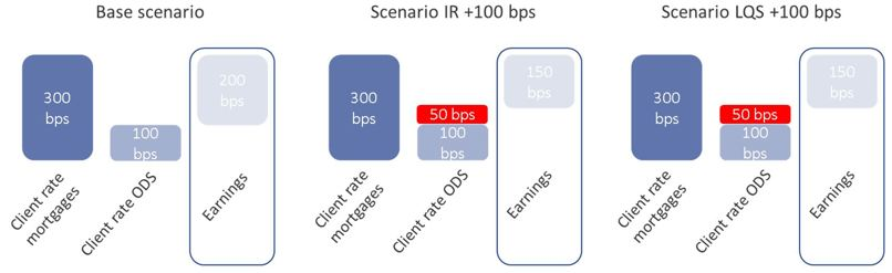
Van Iersel: "Based on newly defined benchmarks, we’ve redefined and shaped our risk appetite as a component part of the strategic program. In the risk appetite process we’ve clarified the difference between how ING wants to manage the IRRBB internally and how the regulator views the type of risk. As a bank, you have to comply with the so-called standard outlier test when it comes to the IRRBB. The benchmark commonly employed for this is the economic value of equity, which is value-based. Within the IRRBB, you can look at the interest rate risk from a value or an income perspective. Both are important, but they occasionally work against one another too. As a bank, we’ve made a choice between them. For us, a constant stream of income was the most important benchmark in defining our interest rate risk strategy, because that’s what is translated to the bottom line of the results that we post. Alongside our internal decision to focus more closely on income and stabilize it, the regulator opted to take a mainly value-based approach. We have explicitly incorporated this distinction in our risk appetite statements. It’s all based on our new strategy; in other words, what we are striving for as a bank and what will be the repercussions for our interest rate risk management. It’s from there that we define the different risk benchmarks."

Which other types of risk does the bank look at and how do they relate to the interest rate risk?

Van Iersel: “From the financial risk perspective, you also have to take into account aspects like credit spreads, changes in the creditworthiness of counterparties, as well as market-related risks in share prices and foreign exchange rates. Given that all these collectively influence our profitability and solvency position, they are also reflected in the Core Tier I ratio. There is a clear link to be seen there between the risk appetite for IRRBB and the overall risk appetite that we as a bank have defined. IRRBB is a component part of the whole, so there’s a certain amount of interaction between them to be considered; in other words, how does the interest rate risk measure up to the credit risk? On top of that, you have to decide where to deploy your valuable capacity. All this has been made clearer in this program.”

Does this mean that every change in the market can be accommodated by adjusting the risk appetite?

Thoolen: “Changing behavior can indeed influence risks and change the risk appetite, although not necessarily. But it can certainly lead to a different use of risk. Moreover, IFRS 9 has changed the accounting standards. Because the Core Tier 1 ratio is based on the accounting standard, these IFRS 9 changes determine the available capital too. If IFRS 9 changes the playing field, it also exerts an influence on certain risk benchmarks.”

In addition to setting up a consistent framework, the standardization of the models used by the different parts of ING was also important. How does ING approach the selection and development of these models?

Thoolen: “With this in mind, we’ve set up a structure with the various business units that we collaborate with from a financial risk perspective. We pay close attention to whether a model is applicable in the environment in which it’s used. In other words, is it a good fit with what’s happening in the market, does it cover all the risks as you see them, and does it have the necessary harmony with the ALM system? In this way, we want to establish optimum modeling for savings or the repayment risk of mortgages, for example.”

But does that also work for an international bank with substantial portfolios in very different countries?

Thoolen: “While there is model standardization, there is no market standardization. Different countries have their own product combinations and, outside the context of IRRBB, have to comply with regulations that differ from other countries. A savings product in the Netherlands will differ from a savings product in Belgium, for example. It’s difficult to define a one-size-fits-all model because the working of one market can be much more specific than another—particularly when it comes to regulations governing retail and wholesale. This sometimes makes standardization more difficult to apply. The challenge lies in the fact that every country and every market is specific, and the differences have to be reconciled in the model.”

Van Iersel: “The model was designed to measure risks as well as possible and to support the business to make good decisions. Having a consistent risk appetite framework can also make certain differences between countries or activities more visible. In Australia, for example, many more floating-rate mortgages are sold than here in the Netherlands, and this alters the sensitivity of the bank’s net interest income when the interest rate changes. Risk appetite statements must facilitate such differences.”

To what extent does the use of machine learning models lead to validation issues?

“Seventy to eighty percent of what we model and validate within the bank is bound by regulation – you can't apply machine learning to that. The kind of machine learning that is emerging now is much more on the business side – how do you find better customers, how do you get cross-selling? You need a framework for that; if you have a new machine learning model, what risks do you see in it and what can you do about it? How do you make sure your model follows the rules? For example, there is a rule that you can't refuse mortgages based on someone's zip code, and in the traditional models that’s well in sight. However, with machine learning, you don't really see what's going on ‘under the hood’. That's a new risk type that we need to include in our frameworks. Another application is that we use our own machine learning models as challenger models for those we get delivered from modeling. This way we can see whether it results in the same or other drivers, or we get more information from the data than the modelers can extract.”

Thoolen: “But opting for a single ALM system imposes this model standardization on you and ensures that, once it’s integrated, it will immediately comply with many conditions. The process is still ongoing, but it’s a good fit with the standardization and consistency that we’re aiming for.”

In conjunction with the changing regulatory environment, the Accelerating Think Forward Strategy formed the backdrop for a major collaboration with Zanders: the IRRBB project. In the context of this project, Zanders researched the extent to which the bank’s interest rate risk framework complied with the changing regulations. The framework also assessed ING’s new interest rate risk benchmarks and best practices. Based on the choices made by the bank, Zanders helped improve and implement the new framework and standardized models in a central risk management system.

At more than 275 years old, Van Lanschot is the oldest independent private bank in the Netherlands. With an eye on the rapidly changing market, last year the bank decided to change its strategy. Evi Van Lanschot is now the young face of the oldest bank and is focusing on the wealthy client of the future.

2013 was an important turning point in Van Lanschot’s development. Under Karl Guha, the new CEO, the bank implemented its new strategy for the coming five years based on three key points: focus, simplification, and growth. “Focus means that we concentrate on what we are really good at, i.e., the retention and growth of our clients’ capital,” explains Martin Van Oort, Van Lanschot’s financial risk management director. “Over the past few years we have increasingly become a ‘small large bank’, with a business banking portfolio. As a result of consolidation in the sector, this will be scaled down even more. As a specialist and independent wealth manager, we think we can really make a difference for our clients.” Customers also wanted simpler and more transparent products. “And we want to extend this line through our organization, in our IT systems and in operations – it has to be simpler and more efficient,” Van Oort continues. “That means rigorous internal reorganization in order to serve our clients in the best possible way. The growth we strive for has to come from the capital management area.”

Synergy with Kempen

Van Lanschot and Kempen are strong labels, which enables the bank to offer a combination of private banking, asset management, and merchant banking. “This offers clients huge advantages; they enjoy an even more tailor-made service,” says Van Oort. The bank’s changed service concept is particularly visible from the outside. For the personal banking segment, Evi Van Lanschot is a clear proposition targeting starters on the capital markets. With the idea that there is private banking potential present, Evi’s entry threshold is much lower. Van Oort says: “Medical specialists and business professionals have differing requirements over the course of their careers and we can assist them in the best possible way over the whole cycle. The Evi bid is going very well; in the Netherlands and Belgium we have approximately €1 billion in savings and managed capital.”

At the same time, clients who currently belong to the personal bank but who require private banking services can – if they pay for it – choose this option. Finally, the bank has a Private Office for extremely wealthy clients. “They too of course profit from the synergy between Van Lanschot and Kempen,” adds Van Oort. Van Lanschot is parting company with another section of the bank – the corporate banking portfolio, which includes commercial real estate financing. “We will do that in a respectable and professional manner. By winding down slowly but retaining service levels, losses can be minimized and clients will have enough time to get a new roof over their heads. Running down this portfolio is going according to plan. We are taking leave of something which no longer fits in with our new strategy and we are putting a lot of effort into private banking. This gives direction and clarity to all of our stakeholders.”

Shorter lines

 All of the bank’s departments are occupied with change. “It’s going well. The shop is open during the reconstruction phase and so customer experience should also stay at a good level. Even the balance sheet ratios – solvability and liquidity – which are so important for the bank, are ahead of our anticipated long-range targets.”

The bank’s culture is changing as well: the traditional bank, where change sometimes appears to be dragging its feet, is becoming younger and more modern. Van Oort explains: “The Evi customer needs a transparent digital service, preferably with a handy fancy app on their mobile. You can see that the bank is also changing in that respect into one with a dynamic culture. For professionals who embrace change, it’s a really great and exciting time. We hear more often that people would like to work for Van Lanschot since so much is happening and we are in the thick of it. Lines are shorter and your ideas have an impact. The fact that it is going well on the personnel front is, of course, important as after all, it is the people who make the bank.”

Parallel to strategy changes, the bank is also investing a good deal in specialist staff functions. Last year it was decided to revise the bank’s risk management; as of March 2013 Van Oort is in charge of a new department – Financial Risk Management. The creation of this department, which was an amalgamation of various teams, was the first step towards further professionalizing risk management. “This second-line department is responsible for consolidated financial risk management within the bank,” he explains. “Besides setting limits and the integral monitoring of the bank’s risk position, this department is also a negotiating partner and advisor to the bank’s senior management.” The department is made up of a group of young and highly educated professionals who are extremely driven. Van Oort adds: “Our traineeships contribute a great deal to recruitment and internal dynamism.”

Forecasting

It is important that the bank is now capable of looking ahead to future developments with the use of forecasting tools. “The classic risk management function of monitoring, reporting and, if necessary, adjusting risk is possible using models and systems, but the world is changing fast – that is a huge challenge,” says Van Oort. “In addition, there is a mountain of rules and regulations that continue to descend on us and which has a great influence on the playing field. As a bank, you have to be more and more critical of the various balance sheet components. Partly because of the low interest rates, it depends on basis points and it is essential to look ahead using various scenarios to see what the impact on the balance sheet ratios and profit could be. The basic model Van Lanschot deployed has to be developed still further, last but not least because of the implementation of Basel III. Therefore, as of 2013, the development of a new forecasting tool was initiated which generates an integrated capital and liquidity forecast based on the expected balance sheet developments. “Zanders made an important contribution here. The good thing about Zanders is that they are real specialists with insight and a lot of practical know-how. But their pragmatic approach also appealed to me. It has resulted in a tool where we can detail the expected development of core ratios and where we can easily and quickly analyze the impact of mitigating measures on these ratios,” Van Oort says. “We are going to continue fine-tuning the good foundations we now have and by constantly carrying out back tests we can see if the forecasts tie in sufficiently. Where necessary, we will adapt the tool. After that, we will further integrate the tool with our ALM systems.”

A more complicated playing field

Van Lanschot is listed on the stock exchange but a large proportion of the shares belong to large financial institutions. “We are active in the capital markets and rating agencies look critically at how our ratios develop and how we cope with risk management. The playing field has become more complicated and the supervisory body also makes its presence felt. Shareholders are of course critical and look at our figures differently to how they did in the past.” The question is whether or not the rapid regulation changes have not overshot their goal in some areas. Van Oort adds: “You see that in the current lending climate: the required growth of capital buffers puts the brakes on possible lending. A new balance has to be found. Extra regulations were necessary, but the amount and complexity of these regulations results in higher costs. Banks’ buffers have increased enormously and also the quality of these buffers has never been so high. The AQR (Asset Quality Review) has confirmed that most banks are on track on this point. Last year it was clear that this was also true of Van Lanschot.” The rating agencies have recently reconfirmed Van Lanschot’s rating, and S&P has upgraded its ‘negative outlook’ to ‘stable’. This is a clear sign that Van Lanschot is on the right track. “It is still closely monitoring the execution of the strategy, in which profitability will be an important factor. Wealth management strategy implies that the interest company reduces in value but is compensated for by increased commissions. In the meantime, we have to maintain our healthy capital and liquidity position. Over the next few years, we will have to prove that the new strategy has been a success.”

Excellent

In the new banking territory, Van Lanschot, with its new strategy, is focusing more than ever on the customer. “Customer satisfaction is up there on top, as it is a very competitive business and for our bank it is essential for us to be an excellent service provider and offer customer value. The strategy we have set out provides a clear answer to how we see ourselves in the future. Within the field of risk management and ALM we are looking for professionals who feel at home in a specialist and dynamic private bank. The added value of our department is to be a sparring partner and advisor to the bank, all the while keeping in mind our penchant for discerning risk. That is a role which will develop along those lines. With all these changes we have a wonderful challenging time ahead of us.”

The Netherlands’ most compact university has a prime location: adjoining the capital’s Zuidas business district and the VU medical center. The VU’s situation is unique in that the city has grown towards it. Both its collaboration with the business sector and with the medical world takes place just a stone’s throw away.

In 1992, the university had approximately 8,000 students; that number is now around 24,000. In terms of the university’s physical real estate, however, not much has been added since the early 1990s. And yet, without any appreciable increase in its accommodation, the number of students studying at the VU has tripled. Partly because of the major growth that the university has experienced, the VU adjusted its substantive vision to the future, under the motto ‘VU Amsterdam: looking further,’ and plans were drafted for expanding or modifying the campus. Since 2003 the university has been considering a vision for the campus; it was only a few years later that it made that vision concrete and the plans for the current renovations on the VU site were established. This gave rise to funding requirements as well.

The early crowd-funders

The VU was founded in 1880 by a group of reformed Protestants, led by Abraham Kuyper. They felt that the education offered at other universities was too liberal. The ties with the reformed Protestant church were strong up until the 1970s. The VU was in fact founded using an early form of crowdfunding: donations from reformed Protestants throughout the Netherlands financed the education at the VU. Fundraisers went door to door asking for donations, carrying green collection boxes bearing a picture of Abraham Kuyper—not only a minister and politician but also known as the founder of the Anti-Revolutionary Party. Radboud University was financed in a similar manner, but by the Catholic community in the Netherlands.

Its original source of funding means the VU has a special structure. While other universities have their roots in the Education Act, the VU is a Dutch stichting (foundation), called the Stichting VU-VUmc, with the university (VU) and medical center (VUmc) as divisions. Other universities such as Leiden University and Utrecht University also work with medical centers, but as separate legal entities and not within a single foundation. “This structure makes it more difficult to arrange funding in the way that other universities do,” says Hanco Gerritse, financial director at the VU. “The VU and VUmc operate as separate entities but must always take each other into account in their financing. In the Netherlands, universities have the possibility of getting funding from the Dutch Ministry of Finance. However, this method of funding, called ‘schatkistbankieren,’ was less attractive in this instance. We therefore chose to work with Zanders, so that the consultants could support us in finding the best financing solution.”

As first university

Zanders first had to investigate how the VU could finance its accommodation plans. Alongside possibilities of bank financing, the VU was also advised to look into a loan via the European Investment Bank (EIB). Gerritse says: “The VU did not have any long-term capital. It was not something we were set up for. Most of the knowledge required we gained from Zanders. And they played an important role in the contact with the EIB. The cooperation fits us like a glove; it is a real partnership.” And the fact that the EIB emerged as a financier is special, says Gerritse. “What makes it so special is that we are the first university in the Netherlands to receive financing from the EIB. Due to both the creditworthiness and nature of the EIB, the pricing is far below those of commercial banks. And they still have more funds available, for the Netherlands and for education in particular.” The construction project involves a total investment of some €460 million. The maximum amount of funding the EIB will provide is half of the investment by way of combined project financing.

Most of the knowledge required we gained from Zanders. And they played an important role in the contact with the EIB. The cooperation fits us like a glove; it is a real partnership.

Hanco Gerritse, financial director at the VU

At other universities, schatkistbankieren and/or loans from commercial banks play a large role in the financing; the VU itself contributes the rest of the investment sum for this project, generated from cash flows and its own resources. These cash flows come from the government, based on the number of students and graduates (the first flow of funds), in the form of research financing (second flow of funds), or originate from the European Union and businesses (third flow of funds). “The buildings used to be owned by the Ministry of Education, but since 1995 the universities own their buildings and sites and are therefore responsible for their accommodation, maintenance, and investments as well,” says Peter Wemmenhove, head of planning & control. “The VU’s main building was built at the beginning of the 1970s and is now in need of renovation. This modernization also falls within the scope of the financing.”

Seven Projects

The projects that fall within the project financing are:

• The O|2 building (due for completion in 2015)
• The Campus square (University building NU.VU)
• New power turbines in the VU’s own power plant: Energy center
• Renovation/upgrade of Main building
• Car park under the O|2 building
• Upgrade of the Medical Faculty building
• Changes to the Mathematics and Physics building

Long-term partnership

Wemmenhove started at the VU in May 2012. The project had already been under way for six months at that point; the information memorandum was being prepared and sent out. Gerritse was appointed financial director one year later. Not long before that he had held the same position at healthcare institution Cordaan, where he also worked on a financing project with Zanders. “We see the EIB’s financing as a show of confidence in our plans from a triple-A-rated European institute,” says Gerritse. “After all, it is a public agency and cannot invest indiscriminately. By investing in our plans, the EIB is endeavoring to achieve the objectives agreed on between the European countries.” The VU and EIB did not only discuss the financial angle; the EIB also cooperated closely with VU’s accommodation department, the Campus Facilities Organization (FCO), and of course the VU medical center.

Zanders also played a big role in that, especially because the process was complicated due to the complex legal structure of the foundation.

Hanco Gerritse, financial director at the VU

The most expensive sports fields

Gerritse proudly explains what buildings are being built with the funds raised: “It is a combined project to build a number of new buildings and overhaul existing buildings. The new buildings will be the O|2 building and the new university building NU.VU. We are also improving the sustainability of all our buildings. For instance, in our own power plant we use seasonal thermal energy storage (STES) to cool or heat the buildings. In the main building, the shell will remain intact and we will open up the many small rooms into larger, brighter open-plan offices. All of which meets the needs of our lecturers and students.” This means more flexible workspaces as well as more opportunities for contact between lecturers and students. “The building must be up to date for at least the next 15 years,” adds Wemmenhove.

Connections between the businesses in the Zuidas district and the university are also being stimulated. “The most expensive sports fields in the Netherlands are across the street,” says Gerritse. “They are owned by the municipality but we are going to trade that land to accomplish a more explicit connection with the city. The sports fields will then be moved to behind our site. This puts us closer to the Zuidas district and brings the businesses even closer to our campus.” So there will be even more cooperation between university, business, and the government—something the government is also eager to encourage.

The VU recently started a major research program in cooperation with the University of Amsterdam and ASML. Some of the laser technology used by the semiconductor manufacturer was developed at the VU. Gerritse adds: “That is a really fine example: conducting research together, using the technological expertise from within the universities and then together finding applications for this knowledge. It has yielded a great deal for Amsterdam. Investing in a strategic partnership makes it easier to achieve such results.”

Phased approach

The VU’s real estate investment is a multi-year plan that runs to 2030. Underlying the multi-year plan is the thinking that the university must find more points of connection with the city: the VU, looking further. “The gates must be open,” says Gerritse. “By establishing the connection with the Zuidas district we can give the entire urban district a boost. That is the larger, urban planning vision behind our plan.”

Within the time span that the European Investment Bank provides funding, seven projects have been defined, both new builds and renovations of existing buildings. These projects comprise the combined project financing for the first phase. The total multi-year plan is executed in different phases. The reason for this phased approach is mainly to limit the risks linked to the investments. “We will examine the situation during every phase,” explains Wemmenhove. “How many students we have, whether the government financing is changing, how business is developing in the Zuidas district—these kinds of factors can prompt us to adjust the course of the plans.” The current investments are still in the first phase and are expected to be completed in 2018. Residential facilities, retail units, and movie theaters are also included in the subsequent phases.

What did Zanders and the VU do together as a
project team?

• The contact with financiers (EIB, commercial banks, and the Ministry of Finance), including negotiations
• Cooperation with FCO (campus facilities organization), VUmc, and Van Doorne (lawyer)
• Drafting of information memorandum, including model and multi-year projections and RfPs
• Selection of financiers
• Structuring of the financing, tailored to the organization and its current financial statements

Better positioned

The funding from the EIB also reflects another trend in the academic world, specifically that universities are becoming increasingly international. The competition between universities is no longer confined by national borders or even by European borders. In the international realm, the city of Amsterdam will also profit from the developments at the VU. “More than half of the master's curricula are in English,” explains Gerritse. “As a university and as a city, you are competing on the international market for higher education. The fact that we have good facilities puts us in a better position in that market as well.” In that sense, too, the financing from the EIB is an affirmation of its confidence. “Compared to a commercial bank, the EIB looks at a financing plan very differently, looking far beyond cash flows and revenue forecasts,” says Koen Reijnders, consultant at Zanders. “Probable questions include, for instance: how will the envisioned building function and how sustainable is it? The EIB only starts looking at the financing component when it’s satisfied from both the engineering viewpoint and the perspective of education economics.”

“We are investing in the Zuidas district,” says Gerritse. “When the VU moved here it was surrounded by farmland that was being sold and bought. Since then, this land has grown into a unique area. The VU had to investigate the right way to develop the space available and, with this plan, we have succeeded in doing this.”