
In order to assess their risk management practices, the Dutch Central Bank (DNB) requires all banks to complete an annual Supervisory Review and Evaluation Process (SREP), including capital and liquidity management self-assessments. To calculate the effect of specific stress test scenarios on the balance sheet and profitability, Delta Lloyd Bank asked Zanders to build a stress test model.
Delta Lloyd Bank is the only bank within the Delta Lloyd Group with a business model which offers mortgages and attracts savings. With a balance sheet of approximately € 5 billion, the bank is a relatively small player in the Dutch banking arena. Delta Lloyd Bank operates in the ever-changing legal and regulatory environment and there is a clear interest to consistently demonstrate how a bank can maintain compliance over the next few years.
Balance sheet projection tool
Delta Lloyd Bank has an asset liability management (ALM) tool which maps out expected mortgage and savings flows. The bank sees how much interest income mortgages generate over a certain time period and when they will be paid back. “We can forecast this for years ahead,” says Andries Broekhuijsen, Teamleader Financial Risk with Delta Lloyd Bank. “Mortgages are calculated at contract level and by using our ALM tool we can also decide if we will grant new mortgages. You get a projection of how the balance sheet will develop. In conjunction with the Business Control department you can calculate a P&L (profit and loss account) for the next five years.” Broekhuijsen adds that the bank then goes a step further. “We have capital ratios, liquidity ratios and several other requirements stemming from the regulatory body. On the basis of the P&L and balance developments we can plot these over time. We have developed an environment where you can see which assumption or development satisfies which regulatory requirement. Also where you don’t comply, and how you can do something about it. For us, within the company, this has become a well-structured process which we use every quarter to forecast one or more years – standard balance sheet forecasting. In the balance sheet projection tool it was not possible to work out different macro-economic scenarios.”
Macro-economic developments
Delta Lloyd Bank wanted to add stress tests to the tool and asked Zanders to help. “The balance sheet projection tool formed the basis for the stress test model which Zanders developed,” Koen Vogels, Actuarial Analyst with Delta Lloyd Bank explains. “There is a sort of extra layer added to the existing tool so when we input certain developments the impact of different scenarios are then presented up clearly and comprehensibly.” Macro-economic developments, like interest rate increases, a drop in house prices or a rise in unemployment, after all, affect the value of the bank’s investments. Vogels: “We needed the insight afforded by the stress tests; what happens with this projection and what are the sensitive issues? Which ratios, for example, change within a certain scenario?”
The balance sheet forecast made by the bank assumes a stable economic situation. “We don’t have an economic office which takes a structural view of economic developments,” Broekhuijsen says. “For our ALM we assume that most economic variables remain constant. In some cases that is not realistic. Using the report Zanders produced, we have been able to develop a number of scenarios based on various economic developments. Unemployment and house prices are very important for us as a mortgage lender. House prices determine how much security we have, while high unemployment can increase the chance of people not being able to pay back their mortgage. Picturing such developments gives us greater insight in our risk profile. We have a relatively high number of NHG mortgages (mortgages which fall under the National Mortgage Guarantee, ed.) and it appears that even if house prices drop substantially we run relatively low risk.”
A more dynamic risk situation
Even though Delta Lloyd Bank has several years of experience carrying out stress tests, they saw room to improve accuracy and efficiency. “How certain macro-economic variables impact relevant risk factors and then the balance sheet is set out in the stress test model. In that way an estimate can be made as to the outcome of the capital and liquidity ratios in specific market circumstances,” says consultant Steyn Verhoeven, who, on behalf of Zanders, helped develop the model. “The model translates certain developments in unemployment figures for example, as an effect on the possibility of payment default by clients. The balance sheet projection tool previously only highlighted one basic scenario, while the stress test model can cover various macro-economic scenarios. This provides the bank with a much wider and more dynamic risk picture. Stress tests not only quantify a minimal capital supply, they instigate discussion on how to deal with negative developments, Verhoeven thinks: “Results from a stress test give management valuable insight into the risk profile of the bank. Which conditions should they be paying the most attention to and what means do they have to turn the tide?”
Scenarios and new assumptions
How do you determine exactly the scenarios you want to understand? Broekhuijsen: “Our basis was the stress test from the EBA (European Banking Authority, ed) and from that we refined the number of scenarios. There is, for example, a ‘baseline scenario’, which is a positive scenario that assumes an increase in house prices. We don’t just look at how bad it can get, but also at improvement.” The problem with developing scenarios is that they have to have enough stress but also tell a useful story, Verhoeven says. “You can make a scenario as extreme as you like, but it does not necessarily furnish the most valuable insights. When developing the stress test model we deliberately opted to work out several scenarios with different stress levels.” A second challenge is the so-called second level effect of a scenario, Broekhuijsen adds. “Take rising interest rates. This results in repricing mortgages; after a certain time the fixed interest period comes to an end and the mortgage rate goes up. But this could also mean that people will want to pay back their mortgage more quickly, because otherwise their costs will increase too much. We have not taken that sort of interactive effect into account, and this is a point needs improvement.”
Reverse stress tests
Over the past few years, regulators have put more focus on stress tests. “Stress tests identify the circumstances when business as usual is no longer enough to keep your organization from dangerous territory,” Broekhuijsen explains. “But if all goes well, this only happens in very extreme circumstances.” As well as a sensitivity analysis and the scenario analysis, many banks carry out reverse stress testing. “You use this to make a recovery plan for a near default, in which you evaluate whether you have taken enough measures to be able to recover. You reason backwards; you determine the ratio of capital unlikely to recover and then investigate which development could cause this to happen. It could be that the credit risk when house prices drop is much lower than the interest rate risk resulting from a drop in interest. Each risk has a different impact,” according to Broekhuijsen.
Complex material
With the aid of the stress test model, Delta Lloyd Bank produces a comprehensive stress test report in a short period of time. Broekhuijsen: “It comprises 15 pages with 5 scenarios and sometimes 20 sensitivity analyses. That is a complete package which we run as soon as we have the quarterly update of our strategic plan. We can show all the issues. The Asset and Liability Commission (ALCO) uses the information to determine if the planned ratio is not too low or too high. That again has an impact on our strategy.” The stress test model also enables the bank to anticipate new regulations. “It is a complex subject,” says Broekhuijsen. “Because there are so many demands made on banks by legal and regulatory bodies, it is difficult to develop a long-term strategy which fulfills these demands. It is therefore very important that we have this tool. We can add all new regulations to the tool and as a result change our strategy; therefore scenarios are restricted to everything which is actually possible and on that basis we can decide on our selection. For example, from IFRS 9, prognoses are more relevant. Elements from the stress test environment are also requested by the regulatory bodies.”
Further integration
Broekhuijsen is happy with the result and the teamwork. “Even the user interface which Zanders built was an eye opener; it is extremely user friendly. We had very little insight and now we have a great starting point. You can do a sensitivity analysis very quickly by using one single variable from the various scenarios in the stress test. We also have other points we can develop, but our emphasis is now on further integration of the stress tests. At the same time we are trying to make the risk picture more dynamic and more interactive.”


Although the general accounting mechanisms will largely remain unchanged, the long waited reforms of IFRS 9 encompass an array of changes that will influence your hedge accounting process in different ways.
Cross-currency interest rate swaps (CC-IRS), options, FX forwards and commodity trades are just a few examples of financial instruments which will be affected by the upcoming changes. The time value, forward points and cross-currency basis spread will receive different accounting treatment under IFRS 9. Within Zanders, we feel the need to clarify these key changes that deserve as much awareness as possible.
1. Accounting for the forward element in foreign currency forwards
Each FX forward contract possesses a spot and forward element. The forward element represents the interest rate differential between the two currencies. Under IFRS 9 (similar to IAS 39), it is allowed to designate the entire contract or just the spot component as the hedging instrument. When designating the spot component only, the change in fair value of the forward element is recognised in OCI and accumulated in a separate component of equity. Simultaneously, the fair value of the forward points at initial recognition is amortised, most expected linearly, over the life of the hedge.
Again, this accounting treatment is only allowed in case the critical terms are aligned (similar). If at inception the actual value of the forward element exceeds the aligned value, changes in the fair value based on the aligned item will go through OCI. The difference between the fair value of the actual and aligned forward elements is recognized in P&L. In case the value of the aligned forward element exceeds the actual value at inception, changes in fair value are based on the lower of aligned versus actual and go to OCI. The remaining change of actual will be recognized in P&L.
Please refer to the example below:
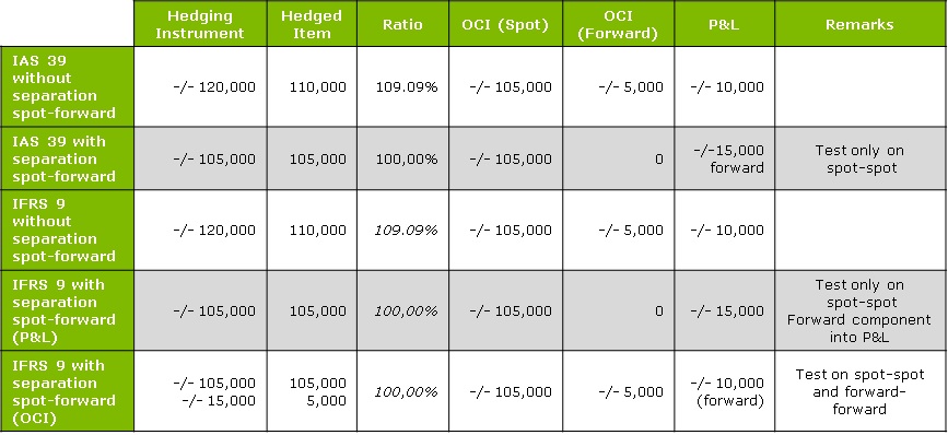
In this example, we consider an entity X which is hedging a future receivable with an FX forward contract.
MtM change of the forward = 105,000 (spot element) + 15,000 (forward element) = 120,000.
MtM change of the hedged item = 105,000 (spot element) + 5,000 (forward element) = 110,000.
We look at alternatives under IAS39 and IFRS9 that show different accounting methods depending on the separation between the spot and forward rates.
Under IAS39 and without a spot/forward separation, the hedging instrument represents the sum of the spot and the forward element (105 000 spot + 15 000 forward= 120 000). The hedged item consisting of 105 000 spot element and 5 000 forward element and the hedge ratio being within the boundaries, the minimum between the hedging instrument and hedged item is listed as OCI, and the difference between the hedging instrument and the hedged item goes to the P&L.
However, with the spot/forward separation under IAS39, the forward component is not included in the hedging relationship and is therefore taken straight to the P&L. Everything that exceeds the movement of the hedged item is considered as an “over hedge” and will be booked in P&L.
Line 3 and 4 under IFRS9 characterise comparable registration practices than under IAS39. The changes come in when we examine line 5, where the forward element of 5 000 can be registered as OCI. In this case, a test on both the spot and the forward element is performed, compared to the previous line where only one test takes place.
2. Rebalancing in a commodity hedge relation
Under influence of changing economic circumstances, it could be necessary to change the hedge ratio, i.e. the ratio between the amount of hedged item and the amount of hedging instruments. Under IAS 39, changes to a hedge ratio require the entity to discontinue hedge accounting and restart with a new hedging relationship that captures the desired changes. The IFRS 9 hedge accounting model allows you to refine your hedge ratio without having to discontinue the hedge relationship. This can be achieved by rebalancing.
Rebalancing is possible if there is a situation where the change in the relationship of the hedging instrument and the hedged item can be compensated by adjusting the hedge ratio. The hedge ratio can be adjusted by increasing or decreasing either the number of designated hedging instruments or hedged items.
When rebalancing a hedging relationship, an entity must update its documentation of the analysis of the sources of hedge ineffectiveness that are expected to affect the hedging relationship during its remaining term.
Please refer to the example below:
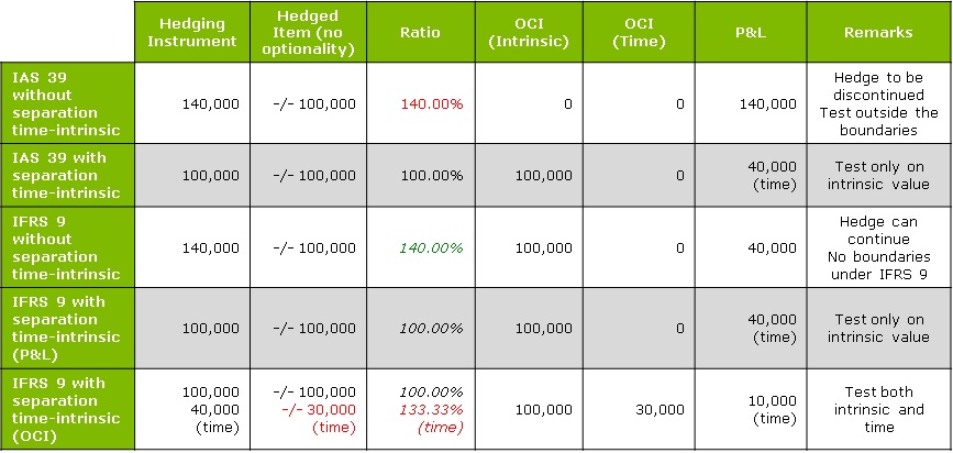
Entity X is hedging a forecast receivable with a FX call.
MtM change of the option = 100,000 (intrinsic value) + 40,000 (time value) = 140,000.
MtM change of the hedged item = 100,000 (intrinsic value) + 30,000 (time value) = 130,000.
In example 3, we consider entity X to be hedging a forecast receivable via an FX call. Note that under IAS39 the hedged item cannot contain an optionality if this optionality is not present in the underlying exposure. Hence, in this example, the hedged item cannot contain any time value. The time value of 30,000 can be used under IFRS9, but only by means of a separate test (see row 5).
In line 1, we can see that without a time-intrinsic separation, the hedge relationship is no longer within the 80-125% boundary; therefore, it needs to be discontinued and the full MtM has to be booked in the P&L. In line 2, there is a time-intrinsic separation, and the 40 000 representing the time value of the option are not included in the hedge relationship, meaning that they go straight to the P&L.
Under IFRS9 with no time-intrinsic separation (line 3), the hedging relationship is accounted for in the usual manner, as the ineffectiveness boundary is not applicable, with 100 000 going representing OCI, and the over hedged 40 000 going to the P&L.
However, the time-intrinsic separation under IFRS9 in line 4 is similar to line 2 under IAS39, in which we choose to immediately remove the time value for the option from the hedging relationship. We therefore have to account for 40 000 of time value in the P&L.
In the last line, we separate between time and intrinsic values, but the time value of the option is aimed to be booked into OCI. In this case, a test on both the intrinsic and the time element is performed. We can therefore comprise 100 000 in the intrinsic OCI, 30 000 in the time OCI, and 10 000 as an over hedge in the P&L.
4. Cross-currency basis spread are considered a cost of hedging
The cross-currency basis spread can be defined as the liquidity premium of one currency over the other. This premium applies to exchanges of currencies in the future, e.g. a hedging instrument like an FX forward contract. If a cross currency interest rate swap is used in combination with a single currency hedged item, for which this spread is not relevant, hedge ineffectiveness could arise.
In order to cope with this mismatch, it has been decided to expand the requirements regarding the costs of hedging. Hedging costs can be seen as cost incurred to protect against unfavourable changes. Similar to the accounting for the forward element of the forward rate, an entity can exclude the cross-currency basis spread and account for it separately when designating a hedging instrument. In case a hypothetical derivative is used, the same principle applies. IFRS 9 states that the hypothetical derivative cannot include features that do not exist in the hedged item. Consequently, cross-currency basis spread cannot be part of the hypothetical derivative in the previously mentioned case. This means that hedge ineffectiveness will exist.
Please refer to the example below:
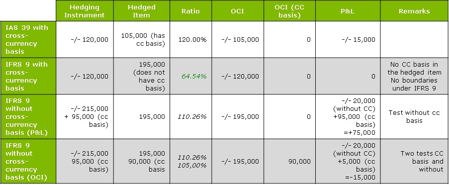
In example 4, we consider an entity X hedging a USD loan with a CCIRS.
MtM change of CCIRS = 215,000 – 95,000 (cross-currency basis) = 120,000.
MtM change hedged = 195,000 – 90,000 (cross-currency basis) = 105,000.
Under IAS39, there is only one way to account for CCIRS. The full amount of 120 000 (including the – 95 000 cross-currency basis) is considered as the hedging instrument, meaning that 105 000 can be listed as OCI and 15 000 of over hedge have to go to the P&L.
Under IFRS9, there is the option to exclude the cross-currency basis and account for it separately.
In line 2, we can see the conditions under IFRS9 when a cross-currency basis is included: the cross-currency basis cannot be comprised in the hedged item, so there is an under hedge of 75 000.
In line 3, we exclude the cross-currency basis from the test for the hedging instrument. By registering the MtM movement of 195 000 as OCI, we then account for the 95 000 of cross-currency basis, as well as -/- 20 000 of over hedge in the P&L. In line 4, the cross-currency basis is included in a separate hedge relationship – we therefore perform an extra test on the cross-currency basis (aligned versus actual values) . From the first test, -/- 195,000 is registered as OCI and -/- 20,000 (“over hedge” part) in P&L; from the cross-currency basis test 90,000 represents OCI and 5,000 has to be included in P&L.

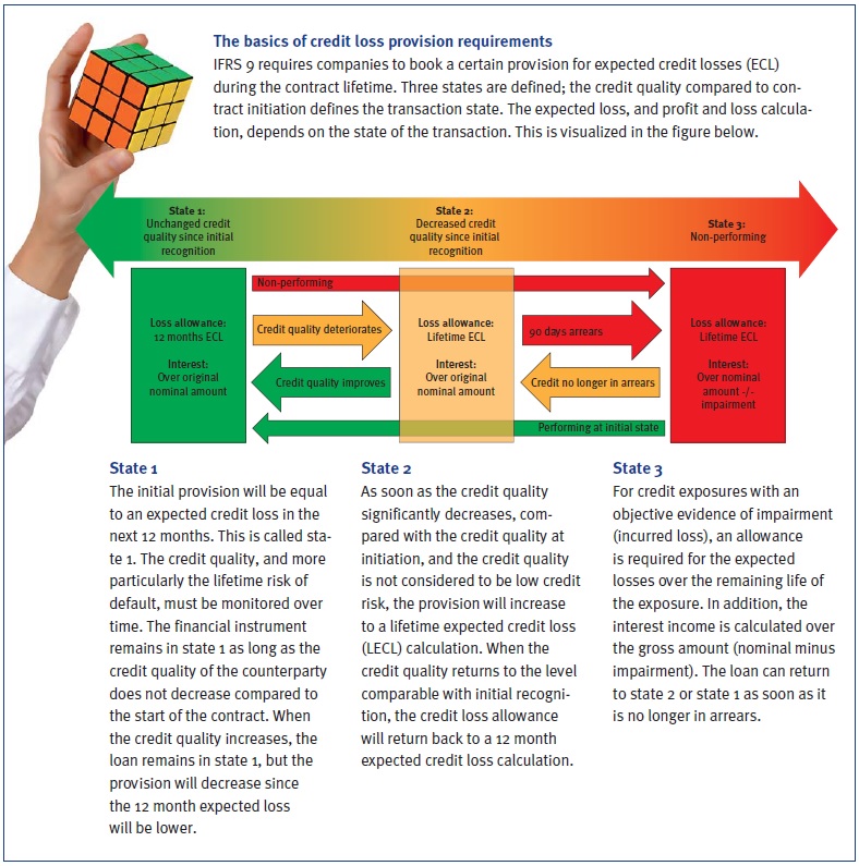
As of January 2018, new accounting rules will come into effect for financial institutions and listed companies with respect to the measurement of impairments. So far, only a few banks act as early adaptors; most choose to be late followers and ‘watch the hare running’. The new rules are principle-based and simple. The design and implementation, however, can be challenging, especially the treatment of forward-looking aspects.
Most banks are struggling to work out how to implement the new impairment rules. Uncertainty over how to deal with current expected credit loss taking into account future macroeconomic scenarios as required by IFRS 9, means credit risk modeling experts, quants and finance experts are in uncharted waters. Different firms have different options on the matter. The primary objective of accounting standards is to provide financial information that stakeholders find useful when making decisions. The new accounting rules regarding provisions will make reserves more timely and sufficient. However, with the new standard, banks are squeezed between P&L volatility, model risk, macroeconomic forecasting and compliance with accounting standards.
Impact
IFRS 9 will, amongst others, rock the balance sheet, affect business models, risk awareness, processes, analytics, data and systems across several dimensions.
We will name a few related to the financials:
- Transition from IAS 39 to IFRS 9 will lead to a change in the level of provision for credit losses. The transition of the current provisions, which are based only on actual losses and incurred but not reported (IBNR) losses, to an expected loss is likely to have significant impact on shareholder equity, net income and capital ratios.
- P&L volatility is expected to increase after transition, since deterioration in credit quality or changes in expected credit loss will have a direct impact on P&L. The P&L volatility will, however, significantly differ per type of credit portfolio, also depending on counterparty ratings and remaining maturity. Portfolios with loans rated below investment grade will move faster from ‘state 1’ to ‘state 2’ (see box), since a move within investment grade ratings is not seen as a credit quality deterioration. Portfolios with long maturities will face large P&L volatility when moving from state 1 to state 2.
- Capital levels and deal pricing will be affected by the expected provisions.
Total P&L over time will not change, since the expected credit loss provision is booked against the actual credit losses during lifetime. If there is no actual credit loss, all provisions will fall free as profit towards maturity.
Forward-looking
IFRS 9 requires financial institutions to adjust the current backward-looking incurred loss based credit provision into a forward-looking expected credit loss. This sounds logical for an accounting provision and it assumes that existing relevant models within risk management may be applied. However, there are some difficulties to overcome.
Incorporating forward-looking information means moving away from the through-the-cycle approach towards an estimation of the ‘business cycle’ of potential credit losses. A forward-looking expected credit loss calculation should be based on an accurate estimation of current and future probability of default (PD), exposure at default (EAD), loss given default (LGD), and discount factors. Discount factors according to IFRS 9 are based on the effective interest rate; this subject will not be further addressed here. The EAD can mainly be derived from current exposure, contractual cash flows and an estimate of unscheduled repayments and an expectation of the use of undrawn credit limits. Both unscheduled repayments and undrawn amounts are known to be business cycle dependent. Forecasting these items can be derived from historical observations.

Of course, the best calibration is on defaulted data since we determine exposure at default. If insufficient data is available, cycle dependent unscheduled repayments and drawing of credit limits can be derived from the entire credit portfolio, preferably corrected with some expert judgement to reflect the situation at default.
Banks have internal rating models in place to assign a PD to a counterparty and for trenching the portfolio in different levels with a specific PD. From a capital point of view, these ratings are mostly calibrated to a through-the-cycle level of observed defaults. Now using all the bank’s forward-looking information may improve estimates if business cycle(s) can be identified, potential scenarios of the development of the cycle in the future can be forecasted, including how the cycle affects a bank’s PD term structure. This would be a macroeconomic and econometric heaven if there were sufficient data available to derive accurate and statistically significant models. Otherwise, banks need to rely more on expert judgement and external macroeconomic reports.
Next to the PD term structures, LGD term structures are required to calculate a life time expected loss. Deriving an accurate LGD term structure from realized defaults requires a large default database. Deriving a business-cycle dependent LGD term structure requires an even bigger database of accurately and timely documented losses. The level of business cycle dependency of LGD significantly differs per type of counterparty, industry, and collateral. Subordination is not much cycle dependent, while loans covered with collateral, such as mortgage loans, may result in large movements in LGDs over time. Hence, this requires different LGD term structures for different LGD types and levels.
Economic scenarios
Incorporating forward-looking information means modeling business cycle dependency in your PD and LGD. For significant drivers, future scenarios are required to calculate expected credit loss. At most banks, these forward-looking scenarios are commonly the domain of economic research departments. Macroeconomic forecasting concentrates mainly on country-specific variables. Growth of domestic product, unemployment rates, inflation indices and interest rates are typical projected variables.
Usually, only large international banks with an economic research department are able to project consistent economic outlooks and scenarios. Next to macro scenarios, industry specific forecasts are important. Industry risk models enable a bank to make forecasts for a certain industry segment, e.g. chemicals, automotive or oil & gas. Industry models are often based on variables such as market conditions, barriers to entry and default data. At some banks, industries are analyzed and scored by economic researchers. At others, usually smaller banks, industries are ranked by sector business specialists.
Industry scorings often form input for rating models and are important factors for portfolio management purposes. Therefore, caution is required in correlation between drivers of ratings and drivers of the PD term structure.
Credit portfolios
For homogenous retail exposures, forward-looking elements can be considered on a portfolio level by modeling the dependencies of PD and LGD percentages for realized defaults and losses; in essence this is a bottom-up approach. For mortgage portfolios, cycle dependency relates, for example, to unemployment and house price indices, among other factors. However, statistically significant parameters and models for default relations are difficult to obtain since there is a common time gap in observing and administrating both defaults and business cycle.
Model significance can be improved by adding additional variables with increasing risk of overfitting. Even if there is statistical proof for macroeconomic dependencies in PD and LGD rates, it is advised to be cautious, since it also requires designing credible macroeconomic scenarios. As business cycles are difficult to predict, this could lead to extra P&L volatility and an increase in the complexity and ‘explainability’ of figures. Therefore, regular back-testing and continuous monitoring are important for an accurate and robust provision mechanism, especially in the first years after the model is introduced.
For non-retail exposures, country and industry risk are, if embedded in the credit rating models, already part of the annual individual credit review and rating assignment processes. In the monthly financial reporting, additional country and industry risk factors can be taken into account on a portfolio basis, making provisions more forward looking; in essence a top-down approach. If necessary, risk management can make adjustments on an individual basis for wholesale counterparties, and facilities. A forward-looking overlay should improve the accuracy of provisions and a timely and adequate recognition of credit risk, instead of “too little, too late” as under the existing rules.
Governance
Because of the forward-looking character of IFRS 9, and the increasing role of risk models, a transparent and robust governance framework will become more important. Coordination and communication are required across risk, finance, business units, audit and IT.
Risk management typically delivers the expected credit loss parameters and calculations to finance on a monthly basis. Proposals for retail and nonretail adjustments briefly described above, must be discussed and agreed upon, after which the final proposal is submitted to the approval authority.
The governance framework should be documented and reviewed on an annual basis, and highlight key functions, stakeholders, definitions, data management, model (re)development, model implementation, portfolio monitoring and validation. In addition, all parties involved should speak the same credit risk language, have access to detailed data underlying the calculation of the provision and a good under- standing of the model and implications of decisions and parametrization. Only then can the finance department obtain an accurate understanding of the level and change of the provision and clearly inform the board and other stakeholders.
Zanders recommends preparing early for IFRS 9 and having a deep and thorough understanding of the impact, as well as the robust tooling and processes in place. Don’t just wait and ‘watch the hare running’, but start early, and at least run a shadow period during daylight to allow sufficient time.
Hassle-free CECL and IFRS9 compliance? Try our new Condor ECL tool!

BNG Bank, established to offer low-rate loans to the Dutch government and public interest institutions, helps lower the cost of public amenities, but its balance sheet’s sensitivity to financial market fluctuations highlights the need for a robust interest rate risk framework.
BNG Bank was founded more than 100 years ago – firstly under the name Gemeentelijke Credietbank – as a purchasing association with the main task of bundling the financing requirements of Dutch local authorities so that purchasing benefits could be obtained on capital markets. In 1922, the name was changed to Bank voor Nederlandsche Gemeenten and even today the main aim is, in essence, the same. What has changed is the role of local authorities, says John Reichardt, a member of the Board of BNG Bank. He explains: “Over the past few years they have diversified. Many of their responsibilities are now independent or even privatized. Hospitals, electricity boards and housing companies, for example, were in the hands of local authorities but now operate independently. They are, however, still our clients because they provide public services.”
Different to Other Banks
To satisfy the financing requirements of its clients, BNG Bank collects money on the international capital markets to realize ‘bundled’ purchasing benefits. “And we pass these benefits on to our customers,” says Reichardt. “While our customers have become more diverse over time, our product portfolio has widened. Some thirty years ago we became a bank, with a comprehensive banking license, and this meant we could take up short-term loans, make investments, and handle our customers’ payments. We try to be a full-service bank, but then only for services our customers need.”
The state holds half of the shares and the remainder belongs to local authorities and provinces/counties. “Because of this we always have the dilemma: should we go for more profit and more dividend, or should our strong purchasing position be reflected immediately in our prices by means of a moderate pricing strategy? Our goal is to be big in our market – we think we should keep 35 to 50 percent of the total outstanding debt on our balance sheet. We are not striving for maximum profit, and that differentiates us from many other banks. Although we are a private company, we do also feel we are a part of the government,” says Reichardt.
Changed Worlds
BNG Bank has only one branch in The Hague, with 300 employees. The bank has grown considerably, mainly over the past few years. As of the start of the financial crisis, a number of services from other parties have disappeared, so BNG Bank was often called upon to step in. Now, partly as a result of this, it has become one of the systematically important Dutch banks. “From a character point of view, we are more of a middle-sized company, but as far as the balance sheet is concerned, we are a large bank. We earn our money by buying cheaply, but also by trying to pass this on as cheaply as possible to our customers – with a small commission. This brings with it a strong focus on risk management, including managing our own assets and the associated risks. These are partly credit risks, but we have fewer risks than other banks – because, thanks to the government, our customers are usually very creditworthy.”
BNG Bank also runs certain interest rate risks that have to be controlled on a day-to-day basis. “We have done this in a certain way for a long time, but in the meantime the world has changed,” says Hans Noordam, head of risk management at BNG Bank. “So we thought it was time to give the method a face-lift to test whether we are doing it right, with the right instruments and whether we are looking at the right things? We also wanted someone else to take a good look at it.”
So BNG Bank concluded that the interest rate risk framework had to be revised. “Our approach once was state of the art but, as always with the dialectics of progress, we didn’t do enough ourselves to keep up with changes in that respect,” Reichardt explains. “When we looked at the whole management of interest rate risk, on the one hand it was about the departments involved, and on the other hand the measurement system – the instruments we used and everything associated with them used to produce information which enabled decision-making on our position strategy. That is a big project.
Project Harry
Over the past few years various developments have taken place in the area of market risk. When BNG Bank changed its products and methods, various changes also took place in the areas of risk management and valuation, including extra requirements from the regulator. “So we started a preliminary investigation and formed one unit within risk management,” says Reichardt. At the end of 2012, BNG Bank appointed Petra Danisevska as head of risk management/ALM (RM/ALM). “We agreed not to reinvent the wheel ourselves, but mainly to look closely at best market practices,” she says.
Zanders helped us with this. In May 2013 we started an investigation to find out which interest rate risks were present in the bank and where improvement levels could be made.
Petra Danisevska, Head of risk management/ALM (RM/ALM) at BNG Bank

Noordam explains that they agreed on suggested steps with the Asset Liability Committee (ALCO), which also provided input and expressed preferences. A plan was then made and the outlines sketched. To convert that into concrete actions, Noordam says that a project was initiated at the beginning of 2014: Project Harry. “This gets its name from BNG Bank’s location, also the home of a Dutch cartoon character, called Haagse Harry. He was the symbol of the whirlwind which was to whip through the bank,” says Noordam.
Within ALCO Limits
“During the (economic) crisis, all sorts of things happened which influenced the valuation of our balance sheet,” Reichardt explains. “They also had many effects on the measurement of our interest rate risk. We had to apply totally different curves – sometimes with very strange results. Our company is set up in a way that with our economic hedging and our hedge accounting, we can buy for X and pass it on to our customers for X plus a couple of basis points, which during the period of the loan reverts to us. We retain a small amount and on the basis of this pay out a dividend – our model is that simple. However, since the valuations were influenced by market changes, we were more or less obliged to take measures in order to stay within our ALCO limits. These measures, with respect to managing our interest position, would not have been realizable under our current philosophy; simply because they weren’t necessary. We knew we had to find a solution for that phenomenon in the project. After much discussion we were able to find a solution: to be more reliable within the technical framework of anticipating market movements which strongly influence valuation of financial instruments. In other words: the spread risk and the rate risk had to be separately measured and managed from one another. The world had changed and our interest rate risk management, as well as reporting and calculations based upon it, had to as well.”
After revision of the interest rate risk framework, as of the second half of 2015, all interest-rate risk measurements, their drivers and reporting were changed. The market risks as a result of the changes in interest rate curves, were then measured and reported on a daily basis by the RM/ALM department. “There is definitely better management of the interest rate risk; we generate more background data and create more possibilities to carry out analyses,” Danisevska explains. “We now have detailed figures that we couldn’t get before, with which we can show ALCO the risk and the accompanying, assumed return.”
More proactive
Noordam knew that Project Harry would involve a considerable effort. “The risk framework would inevitably suffer quite a lot. It had to be innovated on the basis of calculated conditions, while the implementation required a lot of internal resources and specific knowledge. Technical points had to be solved, while relationships had to be safeguarded; many elements with all sorts of expertise had to be integrated. The European Central Bank was stringent – that took up a lot of time and work. We had an asset quality review (AQR) and a stress test – that was completely new to us. Sometimes we were tempted to stay on known ground, but even during those periods we were able to carry on with the project. We rolled up our shirtsleeves and together we gained from the experience.”
Reichardt says: “It was a tough project for us, with complex subject matter and lots of different opinions. In total it took us seven quarters to complete. However, I think we have accomplished more than we expected at the beginning. With a combination of our own people and external expertise, we have managed to make up for lost ground. We have exchanged the rags for riches and we have been successful. Where do we stand now? As well as the required numbers, we have a clear view of what our thoughts are on ‘what is interest rate risk and what isn’t’. The only thing we still have to do is to fine-tune the roles: what can you expect from risk managers and risk takers, and how will they react to this? We will continue to monitor it. RM/ALM as a department is in any case a lot more proactive – that was an important goal for us. We can be more successful, but the department is really earning its spurs within the bank and that means profit for everyone.”

Many banks use a framework of replicating investment portfolios to measure and manage the interest rate risk of variable savings deposits. There are two commonly used methodologies, known as the marginal investment strategy and the portfolio investment strategy. While these have the same objective, the effects for margin and interest maturity may vary. We review these strategies on the basis of a quantitative and a qualitative analysis.
A replicating investment portfolio is a collection of fixed-income investments based on an investment strategy that aims to reflect the typical interest rate maturity of the savings deposits (also referred to as ‘non-maturing deposits’). The investment strategy is formulated so that the margin between the portfolio return and the savings interest rate is as stable as possible, given various scenarios.
A replicating framework enables a bank to base its interest rate risk measurement and management on investments with a fixed maturity and price – while the deposits have no contractual maturity or price. In addition, a bank can use the framework to transfer the interest rate risk from the business lines to the central treasury, by turning the investments into contractual obligations. There are two commonly used methodologies for constructing the replicating portfolios: the marginal investment strategy and the portfolio investment strategy. These strategies have the same objective, but have different effects on margin and interest-rate term, given certain scenarios.
Strategies defined
An investment strategy determines the monthly allocation of the investable volume across various maturities. The investable volume in month t ( It ) consists of two parts:
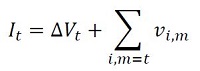
The first part is equal to the decrease or increase in the volume of savings deposits compared to the previous month. The second part is equal to the total principal of all investments in the investment portfolio maturing in the current month (end date m = t ), Σi,m=t vi,m.
By investing or re-investing the volume of these two parts, the total principal of the investment portfolio will equal the savings volume outstanding at that moment. When an investment is generated, it receives the market interest rate relating to the maturity at that time. The portfolio investment return is determined as the principal weighted average interest rate.
The difference between a marginal investment strategy and a portfolio investment strategy is that in a marginal investment strategy, the volume is invested with a fixed allocation across fixed maturities. In a portfolio strategy, these parameters are flexible, however investments are generated in such a way that the resulting portfolio each month has the same (target) proportional maturity profile. The maturity profile provides the total monthly principal of the currently outstanding investments that will mature in the future.
In the savings modeling framework, the interest rate risk profile of the savings portfolio is estimated and defined as a (proportional) maturity profile. For the portfolio investment strategy, the target maturity profile is set equal to this estimated profile. For the marginal investment strategy, the ‘investment rule’ is derived from the estimated profile using a formula. Under long lasting constant or stable volume of savings deposits, the investment portfolio given the investment rule converges to the estimated profile.
Strategies illustrated
In Figure 1, the difference between the two strategies is graphically illustrated in an example. The example provides the development of replicating portfolios of the two strategies in two consecutive months upon increasing savings volume. The replicating portfolios initially consist of the same investments with original maturities of one month, 12 months and 36 months. To this end, the same investments and corresponding principals mature. The total maturing principal will be reinvested and the increase in savings volume will be invested.
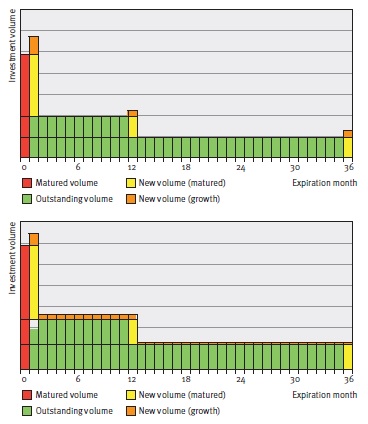
Figure 1: Maturity profiles for the marginal (figure on top) and portfolie (figure below) investment strategies given increasing volume.
Note that if the savings volume would have remained constant, both strategies would have generated the same investments. However, with changing savings volume, the strategies will generate different investments and a different number of investments (3 under the marginal strategy, and 36 under the portfolio strategy).
The interest rate typical maturities and investment returns will therefore differ, even if market interest rates do not change. For the quantitative properties of the strategies, the decision will therefore focus mainly on margin stability and the interest rate typical maturity given changes in volume (and potential simultaneous movements in market interest rates).
Scenario analysis
The quantitative properties of the investment strategies are explained by means of a scenario analysis. The analysis compares the development of the duration, margin and margin stability of both strategies under various savings volume and market interest rate scenarios.
Client interest rate
As part of the simulation of a margin, a client interest rate is modeled. The model consists of a set of sensitivities to market interest rates (M1,t) and moving averages of market interest rates (MA12,t). The sensitivities to the variables show the degree to which the bank has to reflect market movements in its client interest rate, given the profile of its savings clients.
The model chosen for the interest rate for the point in time t (CRt) is as follows:
Up to a certain degree, the model is representative of the savings interest rates offered by (retail) banks.
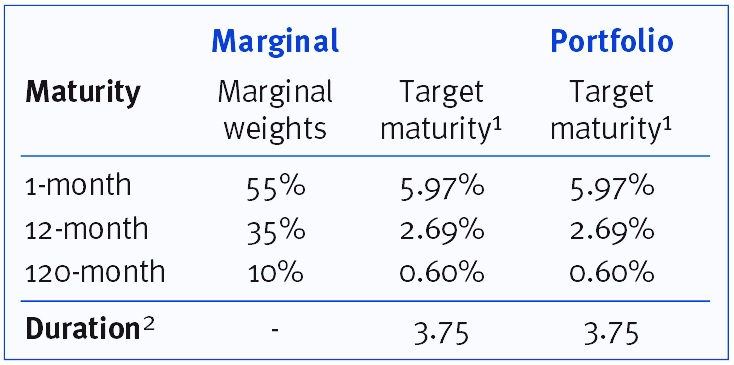
Investment strategies
The investment rules are formulated so that the target maturity profiles of the two strategies are identical. This maturity profile is then determined so that the same sensitivities to the variables apply as for the client rate model. An overview of the investment strategies is given in Table 1.
The replication process is simulated for 200 successive months in each scenario. The starting point for the investment portfolio under both strategies is the target maturity profile, whereby all investments are priced using a constant historical (normal) yield curve. In each scenario, upward and downward shocks lasting 12 months are applied to the savings volume and the yield curve after 24 months.
Example scenario
The results of an example scenario are presented in order to show the dynamics of both investment strategies. This example scenario is shown in Figure 2. The results in terms of duration and margin are shown in Figure 3.
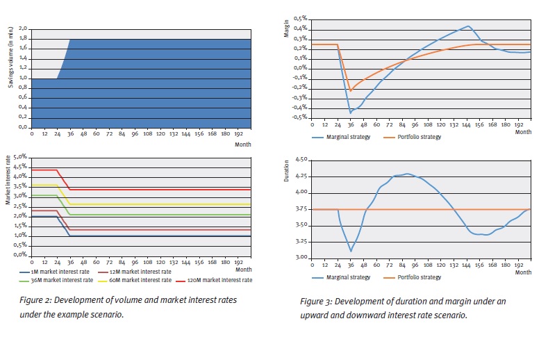
As one would expect, the duration for the portfolio investment strategy remains the same over the entire simulation. For the marginal investment strategy, we see a sharp decline in the duration during the ‘shock period’ for volume, after which a double wave motion develops on the duration. In short, this is caused by the initial (marginal) allocation during the ‘stress’ and subsequent cycles of reinvesting it.
With an upward volume shock, the margin for the portfolio strategy declines because the increase in savings volume is invested at downward shocked market interest rates. After the shock period, the declining investment return and client rate converge. For the marginal strategy this effect also applies and in addition the duration effects feed into the margin development.
Scenario spectrum
In the scenario analysis the standard deviation of the margin series, also known as the margin volatility, serves as a proxy for margin stability. The results in terms of margin stability for the full range of market interest rate and volume scenarios are summarized in Figure 4.
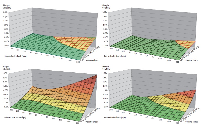
Figure 4: Margin volatility of marginal (left-hand figure) and portfolio strategy (right-hand figure) for upward (above) and downward (below) volume shocks.
From the figures, it can be seen that the margin of the marginal investment strategy has greater sensitivity to volume and interest rate shocks. Under these scenarios the margin volatility is on average 2.3 times higher, with the factor ranging between 1.5 and 4.5. In general, for both strategies, the margin volatility is greatest under negative interest-rate shocks combined with upward or downward volume shocks.
Replication in practice
The scenario analysis shows that the portfolio strategy has a number of advantages over the marginal strategy. First of all, the maturity profile remains constant at all times and equal to the modeled maturity of the savings deposits. Under the marginal strategy, the interest rate typical maturity can vary from it over long periods, even when there are no changes in market interest environment or behavior in the savings portfolio.
Secondly, the development of the margin is more stable under volume and interest rate shocks. The margin volatility under the marginal investment strategy is actually at least one and a half times higher under the chosen scenarios.
An intuitive process
These benefits might, however, come at the expense of a number of qualitative aspects that may form an important consideration when it comes to implementation. Firstly, the advantage of a constant interest-rate profile for the portfolio strategy, comes at the expense of intuitive combinations of investments. This may be important if these investments form contractual obligations for the transfer of the interest rate risk.
The strategy, namely, requires generating a large number of investments that can even have negative principals in case of a (small) decline of savings volume. Secondly, the shocks in the duration in a marginal strategy might actually be desirable and in line with savings portfolio developments. For example, if due to market or idiosyncratic circumstances there is high inflow of deposit volume, this additional volume may be relatively more interest rate sensitive justifying a shorter duration.
Nevertheless, the example scenario shows that after such a temporary decline a temporary increase will follow for which this justification no longer applies.
The choice
A combination of the two strategies may also be chosen as a compromise solution. This involves the use of a marginal strategy whereby interventions trigger a portfolio strategy at certain times. An intervention policy could be established by means of limits or triggers in the risk governance. Limits can be set for (unjustifiable) deviations from the target duration, whereas interventions can be triggered by material developments in the market or the savings portfolio.
In its choice for the strategy, the bank is well-advised to identify the quantitative and qualitative effects of the strategies. Ultimately, the choice has to be in line with the character of the bank, its savings portfolio and the resulting objective of the process.
- The profile shown is a summary of the whole maturity profile. In the whole profile, 5.97% of the replicating volume matures in the first month, 2.69% per month in the second to the 12th month, etc.
- Note that this is a proxy for the duration based on the weighted average maturity of the target maturity profile.
An extended version of this article is published in our Savings Special. Would you like to read it? Please send an e-mail to [email protected].
More articles about ‘The modeling of savings’:

What is their impact and what are the main differences
On April 30th 2014, the European Insurance and Occupational Pensions Authority (EIOPA) published the technical specifications for the preparatory phase towards Solvency II. The technical specifi cations on the long-term guarantee package offer the insurers basically two options to mitigate ‘artificial’ fluctuations in their own funds, the Volatility Adjustment and the Matching Adjustment. What is their impact and what are the main differences between these two measures?
Solvency II aims to unify the EU insurance market and will come into effect on January 1st 2016. The technical specifications published by EIOPA will be used for interim reporting during 2015.
Although the specifications are not yet finalized, it is unlikely that they will change extensively. The technical specifications consist of two parts; part one focuses on the valuation and calculation of the capital requirements and part two focuses on the long-term guarantee (LTG) package. The LTG package was agreed upon in November 2013 and has been one of the key areas of debate in the Solvency II legislation.
Artificial volatility
The LTG package consists of regulatory measures to ensure that short-term market movements are appropriately treated with regards to the long-term nature of the insurance business. It aims to prevent ‘artificial’ volatility in the ‘own funds’ of insurers, while still reflecting the market consistent approach of Solvency II. When insurance companies invest long-term in fixed income markets, they are exposed to credit spread fluctuations not related to an increased probability of default of the counterparty.
These fluctuations impact the market value of the assets and own funds, but not the return of the investments itself as they are held to maturity. The LTG package consists of three options for insurers to deal with this so-called ‘artificial’ volatility: the Volatility Adjustment, the Matching Adjustment and transitional measures.
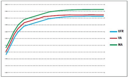
Figure 1
The transitional measures allow insurers to move smoothly from Solvency I to Solvency II and apply to the risk-free curve and technical provisions. However, the most interesting measures are the Volatility Adjustment and the Matching Adjustment. The impact of both measures is difficult to assess and it is a strategic choice which measure should be applied.
Both try to prevent fluctuations in the own funds due to artificial volatility, yet their requirements and use are rather different. To find out more about these differences, we immersed ourselves into the impact of the Volatility Adjustment and the Matching Adjustment.
The Volatility Adjustment
The Volatility Adjustment (VA) is a constant addition to the risk-free curve, which used to calculate the Ultimate Forward Rate (UFR). It is designed to protect insurers with long-term liabilities from the impact of volatility on the insurers’ solvency position. The VA is based on a risk-corrected spread on the assets in a reference portfolio. It is defined as the spread between the interest rate of the assets in the reference portfolio and the corresponding risk-free rate, minus the fundamental spread (which represents default or downgrade risk).
The VA is provided and updated by EIOPA and can differ for each major currency and country. The VA is added to the liquid part of the risk-free zero-coupon rates, i.e. until the so-called Last Liquid Point (LLP). After the LLP, the curve converges to the UFR. The resulting rates are used to produce the relevant risk-free curve.
The Matching Adjustment
The Matching Adjustment (MA) is a parallel shift applied to the entire basic risk-free term structure and serves the same purpose as the VA. The MA is calculated based on the match between the insurers’ assets and the liabilities. The MA is corrected for the fundamental spread. Note that, although the MA is usually higher than the VA, the MA can possibly become negative. The MA can only be applied to a portfolio of life insurance obligations with an assigned portfolio of assets that covers the best estimate of the liabilities.
The mismatch between the cash flows of the assets and the cash flows of the liabilities must not be a material risk in relation to the risks inherent to the insurance business. These portfolios need to be identified, organized and managed separately from other activities of the insurers. Furthermore, the assigned portfolio of assets cannot be used to cover losses arising from other activities of the insurers.
The more of these portfolios are created for an insurance company, the less diversification benefits are possible. Therefore, the MA does not necessarily lead to an overall benefit.
Differences between VA and MA
The main difference between the VA and the MA is that the VA is provided by EIOPA and based on a reference portfolio, while the MA is based on a portfolio of the insurance company.
Other differences include:
- The VA is applied until the LLP, after which the curve converges to the UFR, while the MA is a parallel shift of the whole risk-free curve;
- The MA can only be applied to specifically identified portfolios;
- The VA can be used together with the transitional measures in the preparatory phase, the MA cannot;
- The MA has to be taken into account for the calculation of the Solvency Capital Requirement (SCR) for spread risk. The VA does not respond to SCR shocks for spread risks.
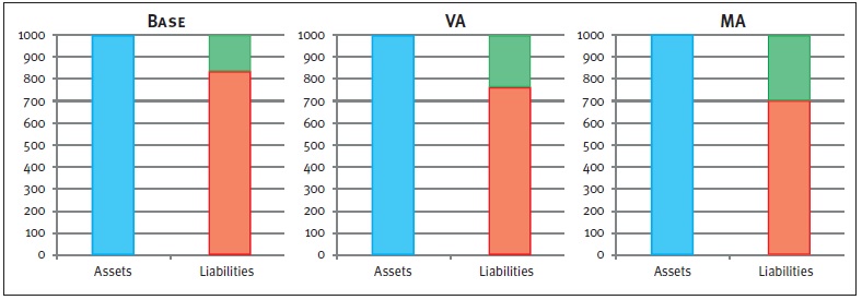
Figure 2: Graphical representations of balance sheets. The blue box represents the assets, the red box the liabilities, and the green box the available capital.
The impact of the VA and MA is twofold. Both adjustments have a direct impact on the available capital and next to this, the MA impacts the SCR. As a result, the level of free capital is affected as well. While the exact impact of the adjustments depends on firm-specific aspects (e.g. cash flows, the asset mix), an indication of the effects on available capital as well as the SCR is given in Figure 2. Please note that this is an example in which all numbers are fictitious and used merely for illustrative purposes.
Impact on available capital
Both the VA and the MA are an addition to the curve used to discount the liabilities, and will therefore lead to an increase in the available capital. The left chart in Figure 2 shows the Base scenario, without adjustment to the risk-free curve. Implementing the VA reduces the market value of the liabilities, but has no effect on the assets. As a result, the available capital increases, which can be seen in the middle chart.
A similar but larger effect can be seen in the right chart, which displays the outcome of the MA. The larger effect on the available capital after the MA compared to the VA is due to two components.
- The MA is usually higher than the VA, and
- the MA is applied to the whole curve.
Impact on the SCR
The calculation of the total SCR, using the Standard Formula, depends on several marginal SCRs. These marginal SCRs all represent a change in an associated risk factor (e.g. spread shocks, curve shifts), and can be seen as the decrease in available capital after an adverse scenario occurs. The risk factors can have an impact on assets, liabilities and available capital, and therefore on the required capital.
Take for example the marginal SCR for spread risk. A spread shock will have a direct, and equal, negative impact on the assets for each scenario. However, since a change in the assets has an impact on the level of the MA, the liabilities are impacted too when the MA is applied. The two left charts in Figure 3 show the results of an increase in the spread, where, by applying the spread shock, the available capital decreases by the same amount (denoted by the striped boxes).
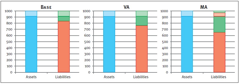
Figure 3: Graphical representations of balance sheets after a positive spread shock. The lined boxes represent a decrease of the corresponding balance sheet item. Note that, in the MA case, the liabilities decrease (striped red box) due to an increase of the MA.
Hence, the marginal SCR for the spread shock will be equal for the Base case and the VA case. The right chart displays an equal effect on the assets. However, the decrease of the assets results in an increase of the MA. Therefore, the liabilities decrease in value too. Consequently, the available capital is reduced to a lesser extent compared to the Base or VA case.
The marginal SCR example for a spread shock clearly shows the difference in impact on the marginal SCR between the MA on the one hand, and the VA and Base case on the other hand. When looking at marginal SCRs driven by other risk factors, a similar effect will occur. Note that the total SCR is based on the marginal SCRs, including diversification effects. Therefore, the impact on the total SCR differs from the sum of the impacts on the marginal SCRs.
Impact on free capital
The impact on the level of free capital also becomes clear in Figure 3. Note that the level of free capital is calculated as available capital minus required capital. It follows directly that the application of either the VA or the MA will result in a higher level of free capital compared to the Base case. Both adjustments initially result in a higher level of available capital.
In addition, the MA may lead to a decrease in the SCR which has an extra positive impact on the free capital. The level of free capital is represented by the solid green boxes in Figure 3. This figure shows that the highest level of free capital is obtained for the MA, followed by the VA and the Base case respectively.
Conclusion
Our example shows that both the VA and the MA have a positive effect on the available capital. Apart from its restrictions and difficulties of the implementation, the MA leads to the greatest benefits in terms of available and free capital.
In addition, applying the MA could lead to a reduction of the SCR. However, the specific portfolio requirements, practical difficulties, lower diversification effects and the possibility of having a negative MA, could offset these benefits.
Besides this, the MA cannot be used in combination with the transitional measures. In order to assess the impact of both measures on the regulatory solvency position for an insurance company, an in-depth investigation is required where all firm specific characteristics are taken into account.

At the Zanders Risk Management seminar last April, after his presentation on ‘Risk management in a changing world’, there didn’t seem to be any questions he couldn’t answer. So we asked Wilfred Nagel, ING Group’s chief risk officer, a few more.
Wilfred Nagel is member of the executive board and chief risk officer (CRO) of the ING Group. He is also CRO of the Management Board Banking. Nagel joined ING in 1996, holding various positions: head of financial engineering at ING Bank, country manager Singapore, head of project & structured finance (Asia), head of regional credit risk management (Asia) and head of regional credit risk management (Americas). In 2002 he was appointed head of group credit risk management, followed by his appointment as CEO of ING wholesale bank Asia in 2005. From 2010, Nagel was CEO of ING Bank Turkey, until he became board member at Bank and Insurance in October 2011. Nagel started his career in 1981 at ABN Amro as a management trainee, after obtaining his degree in economics at VU University in Amsterdam.
This summer, William Coen, secretary general of the Basel Committee, said that the end is nigh for post-crisis reforms to banking regulations, and that the focus is now on implementing them. Do you agree?
"This is probably more wishful thinking than reality. Enthusiasm in politics, the media and academia, and as a spin-off also in the regulatory world, for creating ever stricter rules, has not yet diminished. But at the moment you can’t tell if it’s enough or not. What is important is to stop for a while, implement, look at the impact and then decide what’s missing. What we now have is a continuous introduction of new regulations while previous ones have not yet been implemented or their effect felt. A number of them have a phased timeframe, such as CRD4. The question is: are we giving ourselves enough time to discover what the impact is? The amount of time and work it takes to implement new rules and see what they do for your company is often underestimated. The current dilemma for ordinary banks in most countries is that the savings side is growing faster than the lending side, so there is excess liquidity. The future capital demands for interest risk in the banking book means that longer-term investing can put pressure on the capital position. On the other hand, short-term investment with the current interest rate is bad for results. In fact you should really turn your back on the savers. However that is not in line with our customer-oriented strategy and could eventually cause problems with the NSFR. This is a typical example of how different rules, market conditions and client satisfaction are difficult to unite."
Are Dutch banks still viable after introduction of the CRSA floor (Credit Risk Standardized Approach) which has a significant impact on capital requirements?
“Although I am a risk manager, I am also a bit of an optimist. There is a lot of opposition to the introduction on many fronts, and the impact on economic recovery in Europe could be enormous, so I don’t think that it will be introduced exactly as set out in the consultation papers. But I am fairly sure that something will happen with it and that the average risk weighting adopted will be higher. And then banks with (Dutch) property mortgage portfolios on their balance sheets will be fairly vulnerable. At ING we consider ourselves lucky, because this accounts for about 15% of our global balance sheet – other banks have a much higher percentage. So, can we continue banking? Yes but we will have to change our business model with regards to this point. The business model we use is basically: we grant a loan, keep it on the books for its whole duration and the client pays us back over a period of 15 to 20 years. This is no longer applicable to a large proportion of mortgages. After security checks, they will be passed over more often to institutional investors. The question is, how hungry are investors and how long will it take to turn the balance sheet around to what you want it to be. In the meantime, you, as a bank, are fairly limited in what you can do. Also, the ‘one size fits all’ attitude which is behind the latest proposals could be open to modification. Not everything with the same label is the same. Our Spanish mortgage book for example, is better than the German, Dutch and Belgian ones since in these last three countries a large proportion comes via brokers and in Spain it is only from our own savings clients; we know them. You have to keep your eyes peeled to find the hidden gems. While searching for those gems, we, as a sector, got ahead of ourselves and put too much faith in credit rating agencies such as Standard & Poor’s. But where we do succeed, it’s disappointing to see that the regulators don’t take that into account.”
But ESMA makes it compulsory to work with Moody’s, S&P and Fitch.
“As input it’s fine, but the last step in deciding on a credit rating has to come from the bank itself. Hedge fund critics often overlook the fact that a significant factor in their right to exist comes from being able to give their own independent judgement on a loan, and by doing so can come to other conclusions and other market behavior than the large regulated banks, who find deviating from the norm more difficult. Too much of the same spells danger.”
Although I am a risk manager, I am also a bit of an optimist
Wilfred Nagel, ING Group’s Chief Risk Officer (CRO)
What do you think about the Financial Stability Committee’s proposal for a gradual decrease in the LTV limit (LTV stands for loan-to-value and shows the relationship between the loan and the home value) for mortgages up to 90%?
“I imagine that this is a problem – in this phase of the housing market’s moderate recovery and all the political sensitivity regarding affordable housing for starters. But if you look at it from a normal banker’s perspective, then a prepayment of around 80% on a house is not so strange. The question is whether or not people themselves should take more responsibility for the financial choices they make and their consequences. To save for a number of years and then pay a deposit of 15-20% of the purchase price is not so strange, is it?”
Considering the current low interest levels, is a steep increase in interest not inconceivable at some point? What do you think the consequences will be?
“Banks’ interest margins are under pressure with the current low interest rates. Every time we reinvest the return is less. Up till now banks have been able to compensate in several ways, for example, by lowering savings rates and becoming more efficient. We are also seeing a somewhat increased interest margin by shifting new production to segments with higher spreads, such as project financing and trade financing of certain transfers. At the same time risk costs are showing a gradual improvement in line with economic recovery. The results show that we have been able to manage but decline in the reinvestment returns continues, while there is a limit to what you can do on the savings side. Added to this, the new regulations demand we do relatively more long-term funding. We don’t need this anymore for cash purposes, but we do pay liquidity premiums for it. What is strange is that the traditional balance sheet pattern, where liabilities are a little shorter than assets – the classic gap – is very limited. You see the balance sheet moving more naturally again, but relatively speaking our gap is still much smaller than in a normal interest climate.”
How has ING’s risk management developed since 2008?
"We have focused on mitigating remaining risks that had caused problems during the crisis. Where we ran up against problems was in a couple of large areas, like the Alt-A-portfolio in America, and the project development side of our property company. Our financial markets business also faced hard times, but finally showed a loss for one year only. As far as capital was concerned it has always been self-financing even though the ROI was not very strong. Even so we have radically reduced our trading activities in the financial markets business. An important deciding factor was our expectation that capital demands for this segment would gradually increase. We also looked closely at the global markets in which our position was strong enough to play a significant sustainable role. But the most important exercise since 2008 is that we have rigorously plowed through all large concentrations in the books. When Spain was hit by the euro crisis in 2012, we had EUR 54 billion-worth of assets against about EUR 14 billion-worth of savings. Now we have EUR 28 billion assets and EUR 22 billion savings.”
What impact will the possible introduction of the interest rate risk in the banking book (IRRBB) regulation from Pillar 2 to Pillar 1 have on ING?
“As I said, it will lead to a number of issues for liquidity management and for investment of our capital, which is the longest equity component a bank has. It is not something we are unduly worried about, but it is annoying that it costs capital and work again. Operational costs to comply with the regulations are considerable. The timing is also unfavorable. All banks are busy implementing an integrated finance and risk database. At the same time new regulations have to be implemented which can’t make use of that same database. So all sorts of parallel processes are being run that don’t link in to each other. What we learnt in our AQR (asset quality review) is that it’s not just an adequate database that’s important, but also the ‘query blanket’ on top of it, with which you can define search actions. We have upgraded it for the AQR and are trying to link it to the underlying data stream. We hope to complete the whole process, which was started in 2013, in 2018.”
And what are the priorities for ING for the future?
“The system that collects and invests savings, and another one that produces loans and tries to find funding are going to be more synchronized. We call this strategy ‘one bank’. Collecting franchise money country by country is fine, but if it is at all possible we will have to generate assets ourselves. We want to see a diversified balance sheet per country and are looking more critically at the impact of accounting treatment. If you study our own-generated loan books during the crisis, then they have done well. Of course there is extra pressure on the accounts in a crisis, but that is typical for banking. During the good years you have almost no provisions and a ROI of 20 and in a bad year you have considerably more provision and a ROI of 7. On average you make 13 and everyone is happy. What we have to avoid are large investment portfolios and asset concentrations.”

Van Lanschot is staying ahead of the curve by developing advanced forecasting tools to navigate a rapidly changing financial landscape, ensuring better risk management and adaptability in an increasingly complex regulatory environment.
At more than 275 years old, Van Lanschot is the oldest independent private bank in the Netherlands. With an eye on the rapidly changing market, last year the bank decided to change its strategy. Evi Van Lanschot is now the young face of the oldest bank and is focusing on the wealthy client of the future.
2013 was an important turning point in Van Lanschot’s development. Under Karl Guha, the new CEO, the bank implemented its new strategy for the coming five years based on three key points: focus, simplification, and growth. “Focus means that we concentrate on what we are really good at, i.e., the retention and growth of our clients’ capital,” explains Martin Van Oort, Van Lanschot’s financial risk management director. “Over the past few years we have increasingly become a ‘small large bank’, with a business banking portfolio. As a result of consolidation in the sector, this will be scaled down even more. As a specialist and independent wealth manager, we think we can really make a difference for our clients.” Customers also wanted simpler and more transparent products. “And we want to extend this line through our organization, in our IT systems and in operations – it has to be simpler and more efficient,” Van Oort continues. “That means rigorous internal reorganization in order to serve our clients in the best possible way. The growth we strive for has to come from the capital management area.”
Synergy with Kempen
Van Lanschot and Kempen are strong labels, which enables the bank to offer a combination of private banking, asset management, and merchant banking. “This offers clients huge advantages; they enjoy an even more tailor-made service,” says Van Oort. The bank’s changed service concept is particularly visible from the outside. For the personal banking segment, Evi Van Lanschot is a clear proposition targeting starters on the capital markets. With the idea that there is private banking potential present, Evi’s entry threshold is much lower. Van Oort says: “Medical specialists and business professionals have differing requirements over the course of their careers and we can assist them in the best possible way over the whole cycle. The Evi bid is going very well; in the Netherlands and Belgium we have approximately €1 billion in savings and managed capital.”
At the same time, clients who currently belong to the personal bank but who require private banking services can – if they pay for it – choose this option. Finally, the bank has a Private Office for extremely wealthy clients. “They too of course profit from the synergy between Van Lanschot and Kempen,” adds Van Oort. Van Lanschot is parting company with another section of the bank – the corporate banking portfolio, which includes commercial real estate financing. “We will do that in a respectable and professional manner. By winding down slowly but retaining service levels, losses can be minimized and clients will have enough time to get a new roof over their heads. Running down this portfolio is going according to plan. We are taking leave of something which no longer fits in with our new strategy and we are putting a lot of effort into private banking. This gives direction and clarity to all of our stakeholders.”
Shorter lines
All of the bank’s departments are occupied with change. “It’s going well. The shop is open during the reconstruction phase and so customer experience should also stay at a good level. Even the balance sheet ratios – solvability and liquidity – which are so important for the bank, are ahead of our anticipated long-range targets.”
The bank’s culture is changing as well: the traditional bank, where change sometimes appears to be dragging its feet, is becoming younger and more modern. Van Oort explains: “The Evi customer needs a transparent digital service, preferably with a handy fancy app on their mobile. You can see that the bank is also changing in that respect into one with a dynamic culture. For professionals who embrace change, it’s a really great and exciting time. We hear more often that people would like to work for Van Lanschot since so much is happening and we are in the thick of it. Lines are shorter and your ideas have an impact. The fact that it is going well on the personnel front is, of course, important as after all, it is the people who make the bank.”
Parallel to strategy changes, the bank is also investing a good deal in specialist staff functions. Last year it was decided to revise the bank’s risk management; as of March 2013 Van Oort is in charge of a new department – Financial Risk Management. The creation of this department, which was an amalgamation of various teams, was the first step towards further professionalizing risk management. “This second-line department is responsible for consolidated financial risk management within the bank,” he explains. “Besides setting limits and the integral monitoring of the bank’s risk position, this department is also a negotiating partner and advisor to the bank’s senior management.” The department is made up of a group of young and highly educated professionals who are extremely driven. Van Oort adds: “Our traineeships contribute a great deal to recruitment and internal dynamism.”
Forecasting
It is important that the bank is now capable of looking ahead to future developments with the use of forecasting tools. “The classic risk management function of monitoring, reporting and, if necessary, adjusting risk is possible using models and systems, but the world is changing fast – that is a huge challenge,” says Van Oort. “In addition, there is a mountain of rules and regulations that continue to descend on us and which has a great influence on the playing field. As a bank, you have to be more and more critical of the various balance sheet components. Partly because of the low interest rates, it depends on basis points and it is essential to look ahead using various scenarios to see what the impact on the balance sheet ratios and profit could be. The basic model Van Lanschot deployed has to be developed still further, last but not least because of the implementation of Basel III. Therefore, as of 2013, the development of a new forecasting tool was initiated which generates an integrated capital and liquidity forecast based on the expected balance sheet developments. “Zanders made an important contribution here. The good thing about Zanders is that they are real specialists with insight and a lot of practical know-how. But their pragmatic approach also appealed to me. It has resulted in a tool where we can detail the expected development of core ratios and where we can easily and quickly analyze the impact of mitigating measures on these ratios,” Van Oort says. “We are going to continue fine-tuning the good foundations we now have and by constantly carrying out back tests we can see if the forecasts tie in sufficiently. Where necessary, we will adapt the tool. After that, we will further integrate the tool with our ALM systems.”
A more complicated playing field
Van Lanschot is listed on the stock exchange but a large proportion of the shares belong to large financial institutions. “We are active in the capital markets and rating agencies look critically at how our ratios develop and how we cope with risk management. The playing field has become more complicated and the supervisory body also makes its presence felt. Shareholders are of course critical and look at our figures differently to how they did in the past.” The question is whether or not the rapid regulation changes have not overshot their goal in some areas. Van Oort adds: “You see that in the current lending climate: the required growth of capital buffers puts the brakes on possible lending. A new balance has to be found. Extra regulations were necessary, but the amount and complexity of these regulations results in higher costs. Banks’ buffers have increased enormously and also the quality of these buffers has never been so high. The AQR (Asset Quality Review) has confirmed that most banks are on track on this point. Last year it was clear that this was also true of Van Lanschot.” The rating agencies have recently reconfirmed Van Lanschot’s rating, and S&P has upgraded its ‘negative outlook’ to ‘stable’. This is a clear sign that Van Lanschot is on the right track. “It is still closely monitoring the execution of the strategy, in which profitability will be an important factor. Wealth management strategy implies that the interest company reduces in value but is compensated for by increased commissions. In the meantime, we have to maintain our healthy capital and liquidity position. Over the next few years, we will have to prove that the new strategy has been a success.”
Excellent
In the new banking territory, Van Lanschot, with its new strategy, is focusing more than ever on the customer. “Customer satisfaction is up there on top, as it is a very competitive business and for our bank it is essential for us to be an excellent service provider and offer customer value. The strategy we have set out provides a clear answer to how we see ourselves in the future. Within the field of risk management and ALM we are looking for professionals who feel at home in a specialist and dynamic private bank. The added value of our department is to be a sparring partner and advisor to the bank, all the while keeping in mind our penchant for discerning risk. That is a role which will develop along those lines. With all these changes we have a wonderful challenging time ahead of us.”

Since its introduction in 2012, there has been a great deal of debate about the merits of the Ultimate Forward Rate (UFR). The UFR makes insurers and pension funds less dependent on long-term interest rates and increases funding ratios. However, the recent studies by the Dutch Central Bank (DNB) and the European regulator EIOPA (European Insurance and Occupational Pensions Authority) illustrate that the UFR also brings with it new risks. Does the UFR spell the end of the practical problems associated with market-consistent valuation, or does it actually make them worse?
The UFR is a method of adjusting the market rate at which future commitments are discounted. Interests for durations of more than 20 years are adjusted by converging the one-year forward rate towards the Ultimate Forward Rate of 4.2%.
The introduction of the UFR was an attempt to address three problems. Firstly, as interest rates currently stand, applying the UFR has the effect of increasing rates with a maturity of 20 years or more (see figure 1). This causes the present value of long-term liabilities to fall, which means funding ratios and capital ratios rise. Secondly, the interest rate market for long maturities is assumed to be insufficiently liquid to permit a reliable market valuation, which means the value of liabilities may be very volatile.
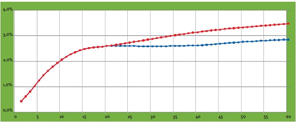
Figure 1: Spot yield curve with UFR (red) and without UFR (blue) as of September 30, 2013
The third problem addressed by the UFR is the desire to escape the vicious circle which is created when interest rate risks are hedged. Due to demand among pension funds and insurers for swaps with long maturities, these interest rates are falling, necessitating further interest rate hedging and triggering a renewed rise in demand.
Risk management
The UFR, however, is raising questions about risk management by insurers and pension funds, who are required to use the UFR when valuing their liabilities in their regulatory reports. From a risk management perspective, however, there are important arguments against hedging interest rate risks on the basis of the UFR.
The UFR is not an economic reality: there are no instruments on the market which generate the same returns as the UFR-adjusted interest rates. Consequently, there is an imbalance between the value as reported to DNB and the available instruments on the market for managing the risks. Furthermore, the UFR is only applied to the liabilities on the balance sheet, and not to the assets. This creates a discrepancy between the economic reality of the assets and the ‘paper’ UFR reality of the liabilities. If a company’s assets and liabilities have identical interest rate profiles, the company does not run an interest rate risk; nonetheless, its UFR-based funding ratio does change in line with interest rate movements on the market. There is also greater interest rate sensitivity around the 20-year interest rate point: past this point, market interest rates are partially or entirely disregarded. Lastly, there is a political risk (which cannot be hedged) that the UFR method may be revised by the regulator – a fact underlined by recent developments.
Insurers and pension funds are compelled to keep two different sets of records: a ‘UFR report’ for the regulator and an economic version on which the interest rate risk is actually managed. Both records have their own, specific risks.
Insurers: debate and uncertainty
Understandably, the UFR has created quite a furor among insurers. In June 2013, EIOPA published the results of a survey of insurers who offer long-term guarantee products. Interestingly, EIOPA acknowledges in this publication that the UFR entails significant risks. Potentially, the UFR could mislead regulators, meaning that any action is taken too late. Moreover, the design of the UFR – specifically, the speed at which the forward rate converges towards the UFR – has long been a source of uncertainty. EIOPA advises using what is known as the ‘20+40’ convergence (whereby market interest rates are used up to and including 20 years and, 40 years later, the forward rate has converged to the UFR). Both insurers and the European Parliament, however, are pressing for a switch to a ‘20+10’ convergence.
Proponents of this shorter convergence period point to the lower sensitivity to shocks in (long-term) market interest rates, which would help stabilize the valuation of liabilities. One drawback of a short convergence period is the increased volatility of own funds. This is because the assets are discounted at market interest rates and are sensitive to changes in interest rates, whereas the liabilities are not. Moreover, the potential impact of a change in the level of the UFR is greater when the convergence period is shorter.
While the debate continues among European insurers, DNB has already compelled Dutch insurers to use the UFR. In so doing, DNB is largely taking its cue from EIOPA’s latest advice. However, there is a high risk that the convergence period will change in the definitive Solvency II legislation, meaning that, eventually, insurers will have to switch to a different UFR.
Pensions: DNB is pursuing its own course
The UFR committee
In October 2013, the UFR committee advised the Dutch cabinet to abandon the current method for pension funds, which involves a fixed UFR of 4.2%. The committee advises using the UFR as an ultimate rate, based on the average forward rates of the last 120 months, with an infinite convergence period.
The UFR will then become a moving target based on current market rates. As things currently stand, this would mean a UFR of 3.9% – which is significantly different to the current UFR.
The cabinet informed the UFR committee in a response that the recommendation of applying a moving target UFR will be implemented from 2015 onwards. This will only accentuate the contrast between Europe and the Dutch pension landscape. In addition to an economic report and the current UFR report, it will compel pension funds to also prepare an adjusted UFR report for 2015.
The situation as regards pension funds illustrates the political risk. Following criticism in Dutch academic circles about the high sensitivity affecting the 20-year forward rate, DNB adapted the rules specifically for pension funds. These funds must now continue applying the forward rate past the 20-year point (with fixed weightings) and the spot rates are averaged over the last three months.
Since then, in its advisory report, the UFR committee has proposed a completely new calculation method (see insert), which may have a big impact on funding ratios. It is not inconceivable that, if the yield curve fluctuates significantly, the UFR will yet again be changed. In addition, there are also long-term risks to be taken into account. The UFR could potentially create discrepancies between the pension entitlements of current and future pensioners.
The higher funding ratio resulting from the application of the UFR reduces the likelihood of increases in contributions and cuts to pensions at the present time – which is an advantage for current pensioners. If, however, the yield turns out lower than assumed, future pensioners will have fewer funds at their disposal. Potentially, therefore, pension rights may end up being transferred from younger to older generations.
Conclusion
The EIOPA study and the UFR committee illustrate that the introduction of the UFR has made the world of insurance more complex. In risk management terms, it has created two landscapes and it is not yet clear exactly what the UFR landscape will look like. From an economic perspective, the majority of risk managers will give priority to hedging risks. To prevent interference by the regulator, however, the UFR value must always be closely monitored. Furthermore, the impending change to the UFR method for pension funds reaffirms that the political risk is a significant, unmanageable factor.

Bank and insurer pay heed to Pento’s perspective
The regulatory changes in the healthcare sector have put smaller establishments with specific care functions in a tight corner. Audiological centers, such as those run by Pento, are among them. In audiological care, the outlay precedes the benefits, yet the bank is setting more stringent financing conditions. How is Pento dealing with this?
The causes of hearing loss are many and varied, from congenital to ‘acquired’ or even psychogenic. Fortunately, thanks to audiological care, there are also many solutions that enable people with hearing impediments to participate in society. The first audiological initiatives in this regard originated in the Netherlands, in the 1960s, when the measurement of hearing using scientific - and therefore reliable - methods became a specialist field in itself. Developments and support in the sphere of language and speech soon followed, because these are closely associated with hearing.
Tensions
In 2007, five audiological centers (AC) decided to merge to form Pento. ‘Penta’ refers to the Greek word for five. There are now six centers and a hearing support service, all located in the central, eastern, and northern areas of the country. Following a referral by a doctor, an AC advises the audiological patient on the appropriate hearing aids and other solutions.
The AC itself does not provide any medical treatment and only employs paramedical staff. Working according to a multidisciplinary approach—which often also involves speech therapy, psychology, and social work—its staff ascertains and analyzes the possible cause of the hearing problem and what can be done about it or offers assistance with the initial use of a hearing aid. The techniques are improving, and hearing impairment is becoming less of a taboo subject.
However, audiological centers too are feeling the effects of the major changes affecting healthcare sector budgets. A free-market system has been introduced along with a new funding system, bringing with it a whole host of changes to the billing process. There are around 30 audiological centers in the Netherlands, a market worth approximately 40 million euros. This means that the audiological sector accounts for less than one percent of the entire healthcare sector. “This is reflected in the tensions that arise whenever you are faced with new government regulations or new policies introduced by health insurers,” explains Jeroen Taalman, director at Pento. “Less account is taken of you. They don’t want to make exceptions to their policies for a small player.” Pento represents a market share of roughly 20% of the audiological sector, making it a big fish in what is a small pond relative to the healthcare sector as a whole. “Consequently, the outside world looks at you differently; people sometimes expect more professionalism in our internal operations than we were able to offer.” The same can be said of Pento’s position and its role as a model within FENAC, the Federation of Dutch Audiological Centers, which represents the centers’ interests. “
In the early years, we took a ‘sticking plaster’ approach to most of our financial decisions,” says Taalman. “So we were often closing the stable door after the horse had bolted, and that was unsustainable. Now, all the necessary arrangements are in place and the structure is clear. We have appointed a financial manager, and an audit committee has been formed, made up of members of the supervisory board. All of which is positive, but our approach remains pragmatic; there are few organizational layers, and we deal with situations as and when they arise. And we are aware that there is a lot more scope for development.”
No capital
What we needed was scenario thinking: what scenarios can we develop for the future and how can we create a future-proof financing structure?
Jeroen Taalman, Director at Pento
The new laws and regulations in the healthcare sector created a quagmire of uncertainties for Pento, chiefly due to the changes in the funding system. “In the space of six months, it all mounted up to such an extent that we felt the ground was slipping away beneath us,” says Taalman. “There were still no contracts in place with health insurers, the fees for each consultation weren’t transparent, and yet we had to calculate the number of consultations we had to reach from a cost perspective. In other words: both the price and the volume were under scrutiny.”
As regards the volume it can achieve, Pento is largely reliant on the referrers, although the law stipulates that various treatments may only be provided by an AC. At the same time, the purchasing ceiling for health insurers means that Pento is only allowed to carry out a maximum number of treatments for a specific fee. Taalman says: “Health insurers are now recognizing that the only way to be able to estimate volume is to form a partnership. The healthcare sector is riddled with inter-dependencies and mutual responsibilities. If we were to suddenly stop or refuse AC care, we would create problems for the health insurer.”
Meanwhile, Pento was contending with another serious financing problem because, until the end of 2011, it was not allowed to build up any equity capital. Under the original funding system, ACs did not generate any profits or losses. Taalman adds: “Being ‘budget-funded’, we had to post a nil result. And if we didn’t, we had to offset the surplus or shortfall against fees the following year. So we were faced with a plethora of rules but weren’t allowed to form any buffers.” This system was dropped in its entirety with effect from 1 January 2012.
Scenario thinking
Back in 2004, FENAC had already warned that if an AC got into financial difficulties, there would be no funds in the coffers to get them out of trouble. Moreover, under the new funding and billing system, ACs would have to finance around half of their annual turnover in advance. Taalman notes: “For a lot of long-term, and therefore expensive, treatments, you can’t send a bill until a year after the first patient visit. So the introduction of a free-market system meant that our bank was also faced with all kinds of uncertainties. As a result, it adopted a very commercially-driven view of us, introducing financial ratios and subjecting them to critical review. A bank expects a certain amount of equity, an order portfolio, and contracts with health insurers. All of which were uncertain factors for us.”
In the spring of 2012, health insurers were locked in negotiations chiefly with the large hospitals. The ACs would follow later. Says Taalman: “They were in no hurry, so we had to ask the bank to keep us afloat. But the bank wasn’t going to readily agree. The bank placed Pento under ‘special management’, setting special, stricter requirements with regard to the provision of information and increasing its risk premiums. We had our backs up against the wall.” Pento felt this problem was becoming too big for it to solve alone. “What we needed was scenario thinking: what scenarios can we develop for the future and how can we create a future-proof financing structure? To do this, you need to bring in outsiders who can think fast and develop models. That’s how we began working with Zanders. It bought us some time with the bank.”
A cure for financial ailments
“Continuity was a very real problem; there were doom scenarios of having to shut down certain Pento centers or services,” says Taalman. “When we were up to our neck in problems, we consciously sought media contact through the newspapers. We were taking a risk, but it opened the health insurers’ eyes. They felt a responsibility to help us.”
During that period, Zanders analyzed the situation and created various scenarios for the financing structure. This went hand in hand with an analysis of internal management and the viability of the Pento organization. The bank then had a clear picture of Pento’s prospects and financing risks. At the same time, Pento was able to conclude contracts with insurers, including a generous advance for the care provided in 2012. These developments earned Pento more time from the bank and led to constructive talks about provisional financing arrangements.
“We were able to work out the impact of the fees and volumes from the contracts on Pento’s liquidity position. Things were soon looking up. In the end, our financial ailments only lasted six months,” Taalman continues. “We now have good arrangements in place with the bank, including regarding the anticipated definitive amount of a residual expense that has to be met in connection with the end of the budget-based funding system, with its adjusted fees. We’re talking a huge sum of money, hardly an amount we can readily afford, so it’s very reassuring that we are now discussing the situation with the bank. It means we can start focusing more on care again, which is our raison d’être.”
Billing for 2012 couldn’t even start until January 2013—a problem affecting the whole of the healthcare sector. Because a new funding and billing system has been introduced, the turnaround times for both healthcare providers and health insurers are even longer. “Billing takes place retrospectively, and yet, historically, Pento has not been able to form any buffers. And that puts huge pressure on your working capital,” explains Zanders’ consultant Marlous Pleijte. “Consequently, agreements have been reached with the bank and the health insurers so that Pento can maintain its working capital at a reasonable level.”
Quality improvements
The agreements have worked for 2012, but the whole palaver is starting again for 2013, says Taalman. “According to the Ministry of Health, Welfare and Sport’s macro-management instrument, from 2010 onwards, the healthcare sector is allowed to grow by a maximum of 2.5% above inflation. The expectation is that we will remain within that limit in 2013, because of the internal budget targets we have set and the highly critical review we have undertaken of our investment policy. Moreover, from 2012 onwards, Pento can build equity capital.”
A number of measures have been taken to enable it to satisfy the bank’s requirements. Pleijte explains: “In the end, we set up a financing structure with a loan portfolio and repayment schedules that work well for Pento, with a clear distinction between working capital and long-term loans. Zanders has also designed some practical tools for managing cash flows and long-term financial planning. Taalman concludes: “This gives us a much better overall picture and, by extension, greater clarity, so we are also better equipped to fulfill our obligations, both internally and vis-à-vis the bank. The result has been a huge improvement in quality. We are now in better shape than ever; business was good last year, and the outlook is healthy. All of which is in stark contrast to the situation a year ago.”


