As sustainability is gaining momentum as a business priority, numerous corporates are re-assessing their business models and strategic goals.
One of the key subjects in this re-assessment is the implementation of tangible and transparent Environment, Social, and Governance (ESG) factors into the business.
Treasury can drive sustainability throughout the company from two perspectives, namely through initiatives within the Treasury function and initiatives promoted by external stakeholders, such as banks, investors, or its clients. When considering sustainability, many treasurers first port of call is to investigate realizing sustainable financing framework. This is driven by the high supply of money earmarked for sustainable goals. However, besides this external focus, Treasury can strive to make its own operations more sustainable and, as a result, actively contribute to company-wide ESG objectives.
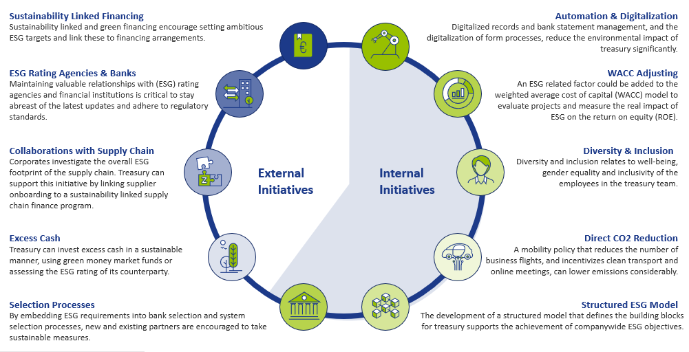
Figure 1: ESG initiatives in scope for Treasury
Treasury holds a unique position within the company because of the cooperation it has with business areas and the interaction with external stakeholders. Treasury can leverage this position to drive ESG developments throughout the company, stay informed of latest updates and adhere to regulatory standards. This article shows how Treasury can become a sustainable support function in its own right, highlights various initiatives within and outside the Treasury department and marks the benefits for Treasury – on top of realising ESG targets.
Internal initiatives
Automation and digitalization drive certain environmental initiatives within the Treasury department. Full digitalized records and bank statement management and the digitalization of form processes reduce the adverse environmental impact of the Treasury department. Besides reducing Treasury’s environmental footprint, digitalization improves efficiency of the Treasury team. By reducing the number of manual, cumbersome operational activities, time can be spent on value-adding activities rather than operational tasks.
Another great example of how Treasury can contribute to the ESG goals of the company, is to incorporate ESG elements in the capital allocation process. This can be done by adding ESG related risk factors to the weighted average cost of capital (WACC) or hurdle investment rates. By having an ESG linked WACC, one can evaluate projects by measuring the real impact of ESG on the required return on equity (ROE). By adjusting the WACC to, for example, the level of CO2 that is emitted by a project, the capital allocation process favours projects with low CO2 emissions.
An additional internal initiative is the design of a mobility policy with the objective to lower CO2 emissions. On one hand, this relates to decreasing the amount of business trips made by the Treasury department itself. On the other hand, it relates to the reduction of business travel by stakeholders of treasury such as bankers, advisors and system vendors. A framework that offsets the added value of a real-life meeting against the CO2 emission is an example of a measure that supports CO2 reduction on both sides. Such a framework supports determination whether the meeting takes place online or in person.
Furthermore, embedding ESG requirements into bank selection, system selection and maintenance processes is a valuable way of encouraging new and existing partners to undertake ESG related measures.
When it comes to social contributions, the focus could be on the diversity and inclusion of the Treasury department, which includes well-being, gender equality and inclusivity of the employees. Pursuing these policies can increase the attractiveness of the organization when hiring talent and make it easier to retain talent within the company, which is also beneficial to the Treasury function.
The development of a structured model that defines the building blocks for Treasury to support the achievement of companywide ESG objectives is a governance initiative that Treasury could undertake. An example of such a model is the Zanders Treasury and Risk Maturity Model, which can be integrated in any organization. This framework supports Treasury in keeping track of its ESG footprint and its contribution to company-wide sustainable objectives. In addition, the Zanders sustainability dashboard provides information on metrics and benchmarks that can be applied to track the progress of several ESG related goals for Treasury. Some examples of these are provided in our ‘Integration of ESG in treasury’ article.
External initiatives
Besides actions taken within the Treasury department, Treasury can boost company-wide ESG performance by leveraging their collaboration with external stakeholders. One of these external initiatives is sustainability linked financing, which is a great tool to encourage the setting of ambitious, company-wide ESG targets and link these to financing arrangements. Examples of sustainability linked financing products include green loans and bonds, sustainability-linked loans, and social bonds. To structure sustainability-linked financing products, corporates often benefit from the guidance of external parties when setting KPIs and ambitious targets and linking these to the existing sustainability strategy. Besides Treasury’s strong relationships with banks, retaining good relationships with (ESG) rating agencies and financial institutions is critical to stay abreast of the latest updates and adhere to regulatory standards. Additionally, investing excess cash in a sustainable manner, using green money market funds or assessing the ESG rating of counterparties, is an effective way of supporting sustainability.
Apart from financing instruments, Treasury can drive the ESG strategy throughout the organization in other ways. Treasury can seek collaborations with business partners to comply with ESG targets, which is another effective manner to achieve ESG related goals throughout the supply chain. An increasing number of corporates is looking to reduce the carbon footprint of their supply chain, for which collaboration is essential. Treasury can support this initiative by linking supplier onboarding on its supply chain finance program to the sustainability performance of suppliers.
To conclude
As developments in ESG are rapidly unfold9ing, Zanders has started an initiative to continuously update our clients to stay ahead of the latest trends. Through the knowledge and network that we have built over the years, we will regularly inform our clients on ESG trends via articles on the news page on our website. The first article will be devoted to the revision of the Sustainability Linked Loan Principles (SLLP) by the Loan Market Association (LMA) and its American and Asian equivalents.
We are keen to hear which topics you would like to see covered. Feel free to reach out to Joris van den Beld or Sander van Tol if you have any questions or want to address ESG topics that are on your agenda.

After the long-acknowledged fact that global warming has catastrophic consequences, it is also increasingly recognized that climate change will impact the financial industry.
The Bank of England is even of the opinion that climate change represents the tragedy of the horizon: “by the time it is clear that climate change is creating risks that we want to reduce, it may already be too late to act” [1]. This article provides a summary of the type of financial risks resulting from climate change, various initiatives within the financial industry relating to the shift towards a low-carbon economy, and an outlook for the assessment of climate change risks in the future.
At the December 2015 Paris Agreement conference, strict measures to limit the rise in global temperatures were agreed upon. By signing the Paris Agreement, governments from all over the world committed themselves to paving a more sustainable path for the planet and the economy. If no action is taken and the emission of greenhouse gasses is not reduced, research finds that per 2100, the temperature will have increased by 3°C to 5°C2.. Climate change affects the availability of resources, the supply and demand for products and services and the performance of physical assets. Worldwide economic costs from natural disasters already exceeded the 30-year average of USD 140 billion per annum in seven out of the last ten years. Extreme weather circumstances influence health and damage infrastructure and private properties, thereby reducing wealth and limiting productivity. According to Frank Elderson, Executive Director at the DNB, this can disrupt economic activity and trade, lead to resource shortages and shift capital from more productive uses to reconstruction and replacement3.
According to the Bank of England, financial risks from climate change come down to two primary risk factors4:
Increasing concerns about climate change has led to a shift in the perception of climate risk among companies and investors. Where in the past analysis of climate-related issues was limited to sectors directly linked to fossil fuels and carbon emissions, it is currently being recognized that climate-related risk exposures concern all sectors, including financials. Banks are particularly vulnerable to climate-related risks as they are tied to every market sector through their lending practices.
Financial risks
- Physical risks. The first risk factor concerns physical risks caused by climate and weather-related events such as droughts and a sea level rise. Potential consequences are large financial losses due to damage to property, land and infrastructure. This could lead to impairment of asset values and borrowers’ creditworthiness. For example, as of January 2019, Dutch financial institutions have EUR 97 billion invested in companies active in areas with water scarcity5. These institutions can face distress if the water scarcity turns into water shortages. Another consequence of extreme climate and weather-related events is the increase in insurance claims: in the US alone, the insurance industry paid out USD 135 billion from natural catastrophes in 2017, almost three times higher than the annual average of USD 49 billion.
- Transition risks. The second risk factor comprises transition risks resulting from the process of moving towards a low-carbon economy. Revaluation of assets because of changes in policy, technology and sentiment could destabilize markets, tighten financial conditions and lead to procyclicality of losses. The impact of the transition is not limited to energy companies: transportation, agriculture, real estate and infrastructure companies are also affected. An example of transition risk is a decrease in financial return from stocks of energy companies if the energy transition undermines the value of oil stocks. Another example is a decrease in the value of real estate due to higher sustainability requirements.
These two climate-related risk factors increase credit risk, market risk and operational risk and have distinctive elements from other risk factors that lead to a number of unique challenges. Firstly, financial risks from physical and transition risk factors may be more far-reaching in breadth and magnitude than other types of risks as they are relevant to virtually all business lines, sectors and geographies, and little diversification is present. Secondly, there is uncertainty in timing of when financial risks may be realized. The possibility exists that the risk impact falls outside of current business planning horizons. Thirdly, despite the uncertainty surrounding the exact impact of climate change risks, combinations of physical and transition risk factors do lead to financial risk. Finally, the magnitude of the future impact is largely dependent on short-term actions.
Initiatives
Many parties in the financial sector acknowledge that although the main responsibility for ensuring the success of the Paris Agreement and limiting climate change lies with governments, central banks and supervisors also have responsibilities. Consequently, climate change and the inherent financial risks are increasingly receiving attention, which is evidenced by the various recent initiatives related to this topic.
Banks and regulators
The Network of Central Banks and Supervisors for Greening the Financial System (NGFS) is an international cooperation between central banks and regulators6. NGFS aims to increase the financial sector’s efforts to achieve the Paris climate goals, for example by raising capital for green and low-carbon investments. NGFS additionally maps out what is needed for climate risk management. DNB and central banks and regulators of China, Germany, France, Mexico, Singapore, UK and Sweden were involved from the start of NGFS in 2017. The ECB, EBA, EIB and EIOPA are currently also part of the network. In the first progress report of October 2018, NGFS acknowledged that regulators and central banks increased their efforts to understand and estimate the extent of climate and environmental risks. They also noted, however, that there is still a long way to go.
In their first comprehensive report of April 2019, NGFS drafted the following six recommendations for central banks, supervisors, policymakers and financial institutions, which reflect best practices to support the Paris Agreement7:
- Integrating climate-related risks into financial stability monitoring and micro-supervision;
- Integrating sustainability factors into own-portfolio management;
- Bridging the data gaps by public authorities by making relevant data to Climate Risk Assessment (CRA) publicly available in a data repository;
- Building awareness and intellectual capacity and encouraging technical assistance and knowledge sharing;
- Achieving robust and internationally consistent climate and environment-related disclosure;
- Supporting the development of a taxonomy of economic activities.
All these recommendations require the joint action of central banks and supervisors. They aim to integrate and implement earlier identified needs and best practices to ensure a smooth transition towards a greener financial system and a low-carbon economy. Recommendations 1 and 5, which are two of the main recommendations, require further substantiation.
- The first recommendation consists of two parts. Firstly, it entails investigating climate-related financial risks in the financial system. This can be achieved by (i) mapping physical and transition risk channels to key risk indicators, (ii) performing scenario analysis of multiple plausible future scenarios to quantify the risks across the financial system and provide insight in the extent of disruption to current business models in multiple sectors and (iii) assessing how to include the consequences of climate change in macroeconomic forecasting and stability monitoring. Secondly, it underlines the need to integrate climate-related risks into prudential supervision, including engaging with financial firms and setting supervisory expectations to guide financial firms.
- The fifth recommendation stresses the importance of a robust and internationally consistent climate and environmental disclosure framework. NGFS supports the recommendations of the Task Force on Climate-related Financial Disclosures (TCFD8) and urges financial institutions and companies that issue public debt or equity to align their disclosures with these recommendations. To encourage this, NGFS emphasizes the need for policymakers and supervisors to take actions in order to achieve a broader application of the TCFD recommendations and the growth of an internationally consistent environmental disclosure framework.
Future deliverables of NGFS consist of drafting a handbook on climate and environmental risk management, voluntary guidelines on scenario-based climate change risk analysis and best practices for including sustainability criteria into central banks’ portfolio management.
Asset managers
To achieve the climate goals of the Paris Agreement, €180 billion is required on an annual basis5. It is not possible to acquire such a large amount from the public sector alone and currently only a fraction of investor capital is being invested sustainably. Research from Morningstar shows that 11.6% of investor capital in the stock market and 5.6% in the bond market is invested sustainably9. Figure 1 shows that even though the percentage of capital invested in sustainable investment funds (stocks and bonds) is growing in recent years, it is still worryingly low.
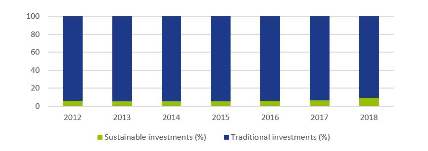
Figure 1: Percentage of invested capital in Europe in traditional and sustainable investment funds (shares and bonds). Source: Morningstar [9].
The current levels of investment are not enough to support an environmentally and socially sustainable economic system. As a result, the European Commission (EC) has raised four initiatives through the Technical Expert Group on sustainable finance (TEG) that are designed to increase sustainable financing10. The first initiative is the issuance of two kinds of green (low-carbon) benchmarks. Offering funds or trackers on these indices would lead to an increase in cash flows towards sustainable companies. Secondly, an EU taxonomy for climate change mitigation and climate change adaptation has been developed. Thirdly, to enable investors to determine to what extent each investment is aligned with the climate goals, a list of economic activities that contribute to the execution of the Paris Agreement has been drafted. Finally, new disclosure requirements should enhance visibility of how investment firms integrated sustainability into their investment policy and create awareness of the climate risks the investors are exposed to.
Insurance firms
Within the insurance sector, the Prudential Regulation Authority (PRA) requires insurers to follow a strategic approach to manage the financial risks from climate change. To support this, in July 2018, the Bank of England (BoE) formed a joint working group focusing on providing practical assistance on the assessment of financial risks resulting from climate changes. In May 2019, the working group issued a six-stage framework that helps insurers in assessing, managing and reporting physical climate risk exposure due to extreme weather events11. Practical guidance is provided in the form of several case studies, illustrating how considering the financial impacts can better inform risk management decisions.
Authorities
Another initiative is the Climate Financial Risk Forum (CFRF), a joint initiative of the PRA and the Financial Conduct Authority (FCA)12. The forum consists of senior representatives of the UK financial sector from banks, insurers and asset managers. CFRF aims to build capacity and share best practices across financial regulators and the industry to enhance responses to the financial climate change risks. The forum set up four working groups focusing on risk management, scenario analysis, disclosure and innovation. The purpose of these working groups, which consist of CFRF members as well as other experts such as academia, is to provide practical guidance on each of the four focus areas.
Current status and outlook
On 5 June 2019, the TCFD published a Status Report assessing a disclosure review on the extent to which 1,100 companies included information aligned with these TCFD recommendations in their 2018 reports. The report also assessed a survey on companies’ efforts to live up to TCFD recommendations and users’ opinion on the usefulness of climate-related disclosures for decision-making13. Based on the disclosure review and the survey, TCFD concluded that, while some of the results were encouraging, not enough companies are disclosing climate change-linked financial information that is useful for decision-making. More specifically, it was found that:
- “Disclosure of climate-related financial information has increased, but is still insufficient for investors;
- More clarity is needed on the potential financial impact of climate-related issues on companies;
- Of companies using scenarios, the majority do not disclose information on the resilience of their strategies;
- Mainstreaming climate-related issues requires the involvement of multiple functions.”
Further, the BoE finds that despite the progress, there is still a long way to go: while many banks are incorporating the most immediate physical risks to their business models and assess exposures to transition risks, many of them are not there yet in their identification and measurement of the financial risks. They stress that governments, financial firms, central banks and supervisors should work together internationally and domestically, private sector and public sector, to achieve a smooth transition to a low-carbon economy. Mark Carney, Governor of the BoE, is optimistic and argues that, conditional on the amount of effort, it should possible to manage the financial climate risks in an orderly, effective and productive manner4.
With respect to the future, Frank Elderson made the following claim: “Now that European banking supervision has entered a more mature phase, we need to retain a forward-looking strategy and develop a long-term vision. Focusing on greening the financial system must be a part of this.”3.
References
1 https://www.bankofengland.co.uk/-/media/boe/files/speech/2019/avoiding-the-storm-climate-change-and-the-financial-system-speech-by-sarah-breeden.pdf
2 https://public.wmo.int/en/media/press-release/wmo-climate-statement-past-4-years-warmest-record
3 https://www.bankingsupervision.europa.eu/press/interviews/date/2019/html/ssm.in190515~d1ab906d59.en.html
4 https://www.bankofengland.co.uk/-/media/boe/files/prudential-regulation/report/transition-in-thinking-the-impact-of-climate-change-on-the-uk-banking-sector.pdf
5 https://fd.nl/achtergrond/1294617/beleggers-moeten-met-de-billen-bloot-over-klimaatrisico-s
6 https://www.dnb.nl/over-dnb/samenwerking/network-greening-financial-system/index.jsp
7 https://www.banque-france.fr/sites/default/files/media/2019/04/17/ngfs_first_comprehensive_report_-_17042019_0.pdf
8 https://www.fsb-tcfd.org/publications/final-recommendations-report/
9 http://www.morningstar.nl/nl/
10 https://ec.europa.eu/info/publications/sustainable-finance-technical-expert-group_en
11 https://www.bankofengland.co.uk/-/media/boe/files/prudential-regulation/publication/2019/a-framework-for-assessing-financial-impacts-of-physical-climate-change.pdf
12 https://www.bankofengland.co.uk/news/2019/march/first-meeting-of-the-pra-and-fca-joint-climate-financial-risk-forum
13 https://www.fsb-tcfd.org/wp-content/uploads/2017/06/FINAL-2017-TCFD-Report-11052018.pdf

Machine learning (ML) models have already been around for decades. The exponential growth in computing power and data availability, however, has resulted in many new opportunities for ML models. One possible application is to use them in financial institutions’ risk management. This article gives a brief introduction of ML models, followed by the most promising opportunities for using ML models in financial risk management.
The current trend to operate a ‘data-driven business’ and the fact that regulators are increasingly focused on data quality and data availability, could give an extra impulse to the use of ML models.
ML models
ML models study a dataset and use the knowledge gained to make predictions for other datapoints. An ML model consists of an ML algorithm and one or more hyperparameters. ML algorithms study a dataset to make predictions, where hyperparameters determine the settings of the ML algorithm. The studying of a dataset is known as the training of the ML algorithm. Most ML algorithms have hyperparameters that need to be set by the user prior to the training. The trained algorithm, together with the calibrated set of hyperparameters, form the ML model.
ML models have different forms and shapes, and even more purposes. For selecting an appropriate ML model, a deeper understanding of the various types of ML that are available and how they work is required. Three types of ML can be distinguished:
- Supervised learning.
- Unsupervised learning.
- Semi-supervised learning.
The main difference between these types is the data that is required and the purpose of the model. The data that is fed into an ML model is split into two categories: the features (independent variables) and the labels/targets (dependent variables, for example, to predict a person’s height – label/target – it could be useful to look at the features: age, sex, and weight). Some types of machine learning models need both as an input, while others only require features. Each of the three types of machine learning is shortly introduced below.
Supervised learning
Supervised learning is the training of an ML algorithm on a dataset where both the features and the labels are available. The ML algorithm uses the features and the labels as an input to map the connection between features and labels. When the model is trained, labels can be generated by the model by only providing the features. A mapping function is used to provide the label belonging to the features. The performance of the model is assessed by comparing the label that the model provides with the actual label.
Unsupervised learning
In unsupervised learning there is no dependent variable (or label) in the dataset. Unsupervised ML algorithms search for patterns within a dataset. The algorithm links certain observations to others by looking at similar features. This makes an unsupervised learning algorithm suitable for, among other tasks, clustering (i.e. the task of dividing a dataset into subsets). This is done in such a manner that an observation within a group is more like other observations within the subset than an observation that is not in the same group. A disadvantage of unsupervised learning is that the model is (often) a black box.
Semi-supervised learning
Semi-supervised learning uses a combination of labeled and unlabeled data. It is common that the dataset used for semi-supervised learning consist of mostly unlabeled data. Manually labeling all the data within a dataset can be very time consuming and semi-supervised learning offers a solution for this problem. With semi-supervised learning a small, labeled subset is used to make a better prediction for the complete data set.
The training of a semi-supervised learning algorithm consists of two steps. To label the unlabeled observations from the original dataset, the complete set is first clustered using unsupervised learning. The clusters that are formed are then labeled by the algorithm, based on their originally labeled parts. The resulting fully labeled data set is used to train a supervised ML algorithm. The downside of semi-supervised learning is that it is not certain the labels are 100% correct.
Setting up the model
In most ML implementations, the data gathering, integration and pre-processing usually takes more time than the actual training of the algorithm. It is an iterative process of training a model, evaluating the results, modifying hyperparameters and repeating, rather than just a single process of data preparation and training. After the training is performed and the hyperparameters have been calibrated, the ML model is ready to make predictions.
Machine learning in financial risk management
ML can add value to financial risk management applications, but the type of model should suit the problem and the available data. For some applications, like challenger models, it is not required to completely explain the model you are using. This makes, for example, an unsupervised black box model suitable as a challenger model. In other cases, explainability of model results is a critical condition while choosing an ML model. Here, it might not be suitable to use a black box model.
In the next section we present some examples where ML models can be of added value in financial risk management.
Data quality analysis
All modeling challenges start with data. In line with the ‘garbage in, garbage out’ maxim, if the quality of a dataset is insufficient then an ML model will also not perform well. It is quite common that during the development of an ML model, a lot of time is spent on improving the data quality. As ML algorithms learn directly from the data, the performance of the resulting model will increase if the data quality increases. ML can be used to improve data quality before this data is used for modeling. For example, the data quality can be improved by removing/replacing outliers and replacing missing values with likely alternatives.
An example of insufficient data quality is the presence of large or numerous outliers. An outlier is an observation that significantly deviates from the other observations in the data, which might indicate it is incorrect. Outlier detection can easily be performed by a data scientist for univariate outliers, but multivariate outliers are a lot harder to identify. When outliers have been detected, or if there are missing values in a dataset, it might be useful to substitute some of these outliers or impute for missing values. Popular imputation methods are the mean, median or most frequent methods. Another option is to look for more suitable values; and ML techniques could help to improve the data quality here.
Multiple ML models can be combined to improve data quality. First, an ML model can be used to detect outliers, then another model can be used to impute missing data or substitute outliers by a more likely value. The outlier detection can either be done using clustering algorithms or by specialized outlier detection techniques.
Loan approval
A bank’s core business is lending money to consumers and companies. The biggest risk for a bank is the credit risk that a borrower will not be able to fully repay the borrowed amount. Adequate loan approval can minimize this credit risk. To determine whether a bank should provide a loan, it is important to estimate the probability of default for that new loan application.
Established banks already have an extensive record of loans and defaults at their disposal. Together with contract details, this can form a valuable basis for an ML-based loan approval model. Here, the contract characteristics are the features, and the label is the variable indicating if the consumer/company defaulted or not. The features could be extended with other sources of information regarding the borrower.
Supervised learning algorithms can be used to classify the application of the potential borrower as either approved or rejected, based on their probability of a future default on the loan. One of the suitable ML model types would be classification algorithms, which split the dataset into either the ‘default’ or ‘non-default’ category, based on their features.
Challenger models
When there is already a model in place, it can be helpful to challenge this model. The model in use can be compared to a challenger model to evaluate differences in performance. Furthermore, the challenger model can identify possible effects in the data that are not captured yet in the model in use. Such analysis can be performed as a review of the model in use or before taking the model into production as a part of a model validation.
The aim of a challenger model is to challenge the model in use. As it is usually not feasible to design another sophisticated model, mostly simpler models are selected as challenger model. ML models can be useful to create more advanced challenger models within a relatively limited amount of time.
Challenger models do not necessarily have to be explainable, as they will not be used in practice, but only as a comparison for the model in use. This makes all ML models suitable as challenger models, even black box models such as neural networks.
Segmentation
Segmentation concerns dividing a full data set into subsets based on certain characteristics. These subsets are also referred to as segments. Often segmentation is performed to create a model per segment to better capture the segment’s specific behavior. Creating a model per segment can lower the error of the estimations and increase the overall model accuracy, compared to a single model for all segments combined.
Segmentation can, among other uses, be applied in credit rating models, prepayment models and marketing. For these purposes, segmentation is sometimes based on expert judgement and not on a data-driven model. ML models could help to change this and provide quantitative evidence for a segmentation.
There are two approaches in which ML models can be used to create a data-driven segmentation. One approach is that observations can be placed into a certain segment with similar observations based on their features, for example by applying a clustering or classification algorithm. Another approach to segment observations is to evaluate the output of a target variable or label. This approach assumes that observations in the same segment have the same kind of behavior regarding this target variable or label.
In the latter approach, creating a segment itself is not the goal, but optimizing the estimation of the target variable or classifying the right label is. For example, all clients in a segment ‘A’ could be modeled by function ‘a’, where clients in segment ‘B’ would be modeled by function ‘b’. Functions ‘a’ and ‘b’ could be regression models based on the features of the individual clients and/or macro variables that give a prediction for the actual target variable.
Credit scoring
Companies and/or debt instruments can receive a credit rating from a credit rating agency. There are a few well-known rating agencies providing these credit ratings, which reflects their assessment of the probability of default of the company or debt instrument. Besides these rating agencies, financial institutions also use internal credit scoring models to determine a credit score. Credit scores also provide an expectation on the creditworthiness of a company, debt instrument or individual.
Supervised ML models are suitable for credit scoring, as the training of the ML model can be done on historical data. For historical data, the label (‘defaulted’ or ‘not defaulted’) can be observed and extensive financial data (the features) is mostly available. Supervised ML models can be used to determine reliable credit scores in a transparent way as an alternative to traditional credit scoring models. Alternatively, credit scoring models based on ML can also act as challenger models for traditional credit scoring models. In this case, explainability is not a key requirement for the selected ML model.
Conclusion
ML can add value to, or replace, models applied in financial risk management. It can be used in many different model types and in many different manners. A few examples have been provided in this article, but there are many more.
ML models learn directly from the data, but there are still some choices to be made by the model user. The user can select the model type and must determine how to calibrate the hyperparameters. There is no ‘one size fits all’ solution to calibrate a ML model. Therefore, ML is sometimes referred to as an art, rather than a science.
When applying ML models, one should always be careful and understand what is happening ‘under the hood’. As with all modeling activities, every method has its pitfalls. Most ML models will come up with a solution, even if it is suboptimal. Common sense is always required when modeling. In the right hands though, ML can be a powerful tool to improve modeling in financial risk management.
Working with ML models has given us valuable insights (see the box below). Every application of ML led to valuable lessons on what to expect from ML models, when to use them and what the pitfalls are.
Machine learning and Zanders
Zanders already encountered several projects and research questions where ML could be applied. In some cases, the use of ML was indeed beneficial; in other cases, traditional models turned out to be the better solution.
During these projects, most time was spent on data collection and data pre-processing. Based on these experiences, an ML based dataset validation tool was developed. In another case, a model was adapted to handle missing data by using an alternative available feature of the observation.
ML was also used to challenge a Zanders internal credit rating model. This resulted in useful insights on potential model improvements. For example, the ML model provided more insight in variable importance and segmentation. These insights are useful for the further development of Zanders’ credit rating models. Besides the insights what could be done better, the ML model also emphasized the advantages of classical models over the ML-based versions. The ML model was not able to provide more sensible ratings than the traditional credit rating model.
In another case, we investigated whether it would be sensible and feasible to use ML for transaction screening and anomaly detection. The outcome of this project once more highlighted that data is key for ML models. The available data was numerous, but of low quality. Therefore, the used ML models were not able to provide a helpful insight into the payments, or to consistently detect divergent payment behavior on a large scale.
Besides the projects where ML was used to deliver a solution, we investigated the explainability of several ML models. During this process we gained knowledge on techniques to provide more insights into otherwise hardly understandable (black box) models.

Zanders add-on for SAP TRM – An Average Rate FX Forward (ARF) can be a very efficient hedging instrument when the business margin needs to be protected. It allows the buyer to hedge the outright rate in a similar way as with a regular forward. However, as the cash settlement amount is calculated against the average of spot rates observed over an extended period, the volatility of the pay-out is much reduced.
The observation period for the average rate calculation is usually long and can be defined flexibly with daily, weekly or monthly periodicity. Though this type of contract is always settled as non-delivery forward in cash, it is a suitable hedging instrument in certain business scenarios, especially when the underlying FX exposure amount cannot be attributed to a single agreed payment date. In case of currencies and periods with high volatility, ARF reduces the risk of hitting an extreme reading of a spot rate.
Business margin protection
ARF can be a very efficient hedging instrument when the business margin needs to be protected, namely in the following business scenarios:
- Budgeted sales revenue or budgeted costs of goods sold are incurred with reliable regularity and spread evenly in time. This exposure needs to be hedged against the functional currency.
- The business is run in separate books with different functional currencies, FX exposure is determined and hedged against the respective functional currency of these books. Resulting margin can be budgeted with high degree of reliability and stability, is relatively small and needs to be hedged from the currency of the respective business book to the functional currency of the reporting entity.
Increased complexity
Hedging such FX exposure with conventional FX forwards would lead to a very high number of transactions, as well as data on the side of underlying FX exposure determination, resulting in a data flood and high administrative effort. A hedge accounting according the IFRS 9 rules is almost impossible due to high number of hedge relationships to manage. The complexity increases even more if treasury operations are centralized and the FX exposure has to be concentrated via intercompany FX transactions in the group treasury first.
If the ARF instruments are not directly supported by the used treasury management system (TMS), the users have to resort to replicating the single external ARF deal with a series of conventional FX forwards, creating individual FX forwards for each fixation date of the observation period. As the observation periods are usually long (at least 30 days) and rate fixation periodicity is usually daily, this workaround leads to a high count of fictitious deals with relatively small nominal, leading to an administrative burden described above. Moreover, this workaround prevents automated creation of deals via an interface from a trading platform and automated correspondence exchange based on SWIFT MT3xx messages, resulting in a low automation level of treasury operations.
Add-on for SAP TRM
Currently, the ARF instruments are not supported in SAP Treasury and Risk management system (SAP TRM). In order to bridge the gap and to help the centralized treasury organizations to further streamline their operations, Zanders has developed an add-on for SAP TRM to manage the fixing of the average rate over the observation period, as well as to correctly calculate the fair value of the deals with partially fixed average rate.
The solution consists of dedicated average rate FX forward collective processing report, covering:
- Particular information related to ARF deals, including start and end of the fixation period, currently fixed average rate, fixed portion (percentage), locked-in result for the fixed portion of the deal in the settlement currency.
- Specific functions needed to manage this type of deals: creation, change, display of rate fixation schedule, as well as creating final fixation of the FX deal, once the average rate is fully calculated through the observation period.
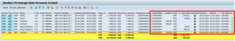
Figure 1 Zanders FX Average Rate Forwards Cockpit and the ARF specific key figures
The solution builds on the standard SAP functionality available for FX deal management, meaning all other proven functionalities are available, such as payments, posting via treasury accounting subledger, correspondence, EMIR reporting, calculation of fair value for month-end evaluation and reporting. Through an enhancement, the solution is fully integrated into market risk, credit risk and, if needed, portfolio analyser too. Therefore, correct mark-to-market is always calculated for both the fixed and unfixed portion of the deal.
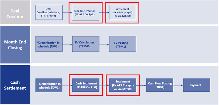
Figure 2 Integration of Zanders ARF solution into SAP Treasury Transaction manager process flow
The solution builds on the standard SAP functionality available for FX deal management, meaning all other proven functionalities are available, such as payments, posting via treasury accounting subledger, correspondence, EMIR reporting, calculation of fair value for month-end evaluation and reporting. Through an enhancement, the solution is fully integrated into market risk, credit risk and, if needed, portfolio analyser too. Therefore, correct mark-to-market is always calculated for both the fixed and unfixed portion of the deal.
Zanders can support you with the integration of ARF forwards into your FX exposure management process. For more information do not hesitate to contact Michal Šárnik.

Managing Capital Adequacy ratios through an open Foreign Exchange position
Since the introduction of the Pillar 1 capital charge for market risk, banks must hold capital for Foreign Exchange (FX) risk, irrespective of whether the open FX position was held on the trading or the banking book. An exception was made for Structural Foreign Exchange Positions, where supervisory authorities were free to allow banks to maintain an open FX position to protect their capital adequacy ratio in this way.
This exemption has been applied in a diverse way by supervisors and therefore, the treatment of Structural FX risk has been updated in recent regulatory publications. In this article we discuss these publications and market practice around Structural FX risk based on an analysis of the policies applied by the top 25 banks in Europe.
Based on the 1996 amendment to the Capital Accord, banks that apply for the exemption of Structural FX positions can exclude these positions from the Pillar 1 capital requirement for market risk. This exemption was introduced to allow international banks with subsidiaries in currencies different from the reporting currency to employ a strategy to hedge the capital ratio from adverse movements in the FX rate. In principle a bank can apply one of two strategies in managing its FX risk.
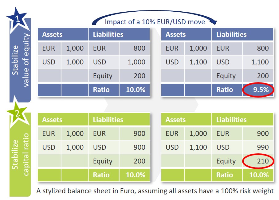
- In the first strategy, the bank aims to stabilize the value of its equity from movements in the FX rate. This strategy requires banks to maintain a matched currency position, which will effectively protect the bank from losses related to FX rate changes. Changes in the FX rate will not impact the equity of a bank with e.g. a consolidated balance sheet in Euro and a matched USD position. The value of the Risk-Weighted Assets (RWAs) is however impacted. As a result, although the overall balance sheet of the bank is protected from FX losses, changes in the EUR/USD exchange rate can have an adverse impact on the capital ratio.
- In the alternative strategy, the objective of the bank is to protect the capital adequacy ratio from changes in the FX rate. To do so, the bank deliberately maintains a long, open currency position, such that it matches the capital ratio. In this way, both the equity and the RWAs of the bank are impacted in a similar way by changes in the EUR/USD rate, thereby mitigating the impact on the capital ratio. Because an open position is maintained, FX rate changes can result in losses for the bank. Without the exemption of Structural FX positions, the bank would be required to hold a significant amount of capital for these potential losses, effectively turning this strategy irrelevant.
As can also be seen in the exhibit below, the FX scenario that has an adverse impact on the bank differs between both strategies. In strategy 1, an appreciation of the currency will result in a decrease of the capital ratio, while in the second strategy the value of the equity will increase if the currency appreciates. The scenario with an adverse impact on the bank in strategy 2 is when the foreign currency depreciates.
Until now, only limited guidance has been available on e.g. the risk management framework, (number of) currencies that can be in scope of the exemption and the maximum open exposure that can be exempted. As a result, the practical implementation of the Structural FX exemption varies significantly across banks. Recent regulatory publications aim to enhance regulatory guidance to ensure a more standardized application of the exemption.
Regulatory Changes
With the publication of the Fundamental Review of the Trading Book (FRTB) in January 2019, the exemption of Structural FX risk was further clarified. The conditions from the 1996 amendment were complemented to a total of seven conditions related to the policy framework required for FX risk and the maximum and type of exposure that can be in scope of the exemption. Within Europe, this exemption is covered in the Capital Requirements Regulation under article 352(2).
To process the changes introduced in the FRTB and to further strengthen the regulatory guidelines related to Structural FX, the EBA has issued a consultation paper in October 2019. A final version of these guidelines was published in July 2020. The date of application was pushed back one year compared to the consultation paper and is now set for January 2022.
The guidelines introduced by EBA can be split in three main topics:
- Definition of Structural FX.
The guidelines provide a definition of positions of a structural nature and positions that are eligible to be exempted from capital. Positions of a structural nature are investments in a subsidiary with a reporting currency different from that of the parent (also referred to as Type A), or positions that are related to the cross-border nature of the institution that are stable over time (Type B). A more elaborate justification is required for Type B positions and the final guidelines include some high-level conditions for this. - Management of Structural FX.
Banks are required to document the appetite, risk management procedures and processes in relation to Structural FX in a policy. Furthermore, the risk appetite should include specific statements on the maximum acceptable loss resulting from the open FX position, on the target sensitivity of the capital ratios and the management action that will be applied when thresholds are crossed. It is moreover clarified that the exemption can in principle only be applied to the five largest structural currency exposures of the bank. - Measurement of Structural FX.
The guidelines include requirements on the type and the size of the positions that can be in scope of the exemption. This includes specific formulas on the calculation of the maximum open position that can be in scope of the exemption and the sensitivity of the capital ratio. In addition, banks will need to report the structural open position, maximum open position, and the sensitivity of the capital ratio, to the regulator on a quarterly basis.
One of the reasons presented by the EBA to publish these additional guidelines is a growing interest in the application of the Structural FX exemption in the market.
Market Practice
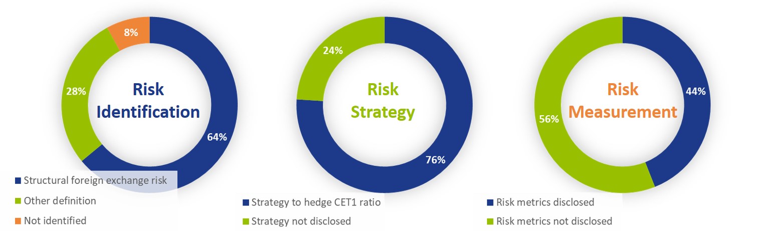
To understand the current policy applied by banks, a review of the 2019 annual reports of the top 25 European banks was conducted. Our review shows that almost all banks identify Structural FX as part of their risk identification process and over three quarters of the banks apply a strategy to hedge the CET1 ratio, for which an exemption has been approved by the ECB. While most of the banks apply the exemption for Structural FX, there is a vast difference in practices applied in measurement and disclosure. Only 44% of the banks publish quantitative information on Structural FX risk, ranging from the open currency exposure, 10-day VaR losses, stress losses or Economic Capital allocated.
The guideline that will have a significant impact on Structural FX management within the bigger banks of Europe is the limit to include only the top five open currency positions in the exemption: of the banks that disclose the currencies in scope of the Structural FX position, 60% has more than 5 and up to 20 currencies in scope. Reducing that to a maximum of five will either increase the capital requirements of those banks significantly or require banks to move back to maintaining a matched position for those currencies, which would increase the capital ratio volatility.
Conclusion
The EBA guidelines on Structural FX that will to go live by January 2022 are expected to have quite an impact on the way banks manage their Structural FX exposures. Although the Structural FX policy is well developed in most banks, the measurement and steering of these positions will require significant updates. It will also limit the number of currencies that banks can identify as Structural FX position. This will make it less favourable for international banks to maintain subsidiaries in different currencies, which will increase the cost of capital and/or the capital ratio volatility.
Finally, a topic that is still ambiguous in the guidelines is the treatment of Structural FX in a Pillar 2 or ICAAP context. Currently, 20% of the banks state to include an internal capital charge for open structural FX positions and a similar amount states to not include an internal capital charge. Including such a capital charge, however, is not obvious. Although an open FX position will present FX losses for a bank which would favour an internal capital charge, the appetite related to internal capital and to the sensitivity of the capital ratio can counteract, resulting in the need for undesirable FX hedges.
The new guidelines therefore present clarifications in many areas but will also require banks to rework a large part of their Structural FX policies in the middle of a (COVID-19) crisis period that already presents many challenges.

The Swiss Average Rate Overnight (SARON) is expected to replace CHF LIBOR by the end of 2021. The transition to this new reference rate includes debates concerning the alternative methodologies for compounding SARON. This article addresses the challenges associated with the compounding alternatives.
In our previous article, the reasons for a new reference rate (SARON) as an alternative to CHF LIBOR were explained and the differences between the two were assessed. One of the challenges in the transition to SARON, relates to the compounding technique that can be used in banking products and other financial instruments. In this article the challenges of compounding techniques will be assessed.
Alternatives for a calculating compounded SARON
After explaining in the previous article the use of compounded SARON as a term alternative to CHF LIBOR, the Swiss National Working Group (NWG) published several options as to how a compounded SARON could be used as a benchmark in banking products, such as loans or mortgages, and financial instruments (e.g. capital market instruments). Underlying these options is the question of how to best mitigate uncertainty about future cash flows, a factor that is inherent in the compounding approach. In general, it is possible to separate the type of certainty regarding future interest payments in three categories . The market participant has:
- an aversion to variable future interest payments (i.e. payments ex-ante unknown). Buying fixed-rate products is best, where future cash flows are known for all periods from inception. No benchmark is required due to cash flow certainty over the lifetime of the product.
- a preference for floating-rate products, where the next cash flow must be known at the beginning of each period. The option ‘in advance’ is applicable, where cash flow certainty exists for a single period.
- a preference for floating-rate products with interest rate payments only close to the end of the period are tolerated. The option ‘in arrears’ is suitable, where cash flow certainty only close to the end of each period exists.
Based on the Financial Stability Board (FSB) user’s guide, the Swiss NWG recommends considering six different options to calculate a compounded risk-free rate (RFR). Each financial institution should assess these options and is recommended to define an action plan with respect to its product strategy. The compounding options can be segregated into options where the future interest rate payments can be categorized as in arrears, in advance or hybrid. The difference in interest rate payments between ‘in arrears’ and ‘in advance’ conventions will mainly depend on the steepness of the yield curve. The naming of the compounding options can be slightly different among countries, but the technique behind those is generally the same. For more information regarding the available options, see Figure 1.
Moreover, for each compounding technique, an example calculation of the 1-month compounded SARON is provided. In this example, the start date is set to 1 February 2019 (shown as today in Figure 1) and the payment date is 1 March 2019. Appendix I provides details on the example calculations.
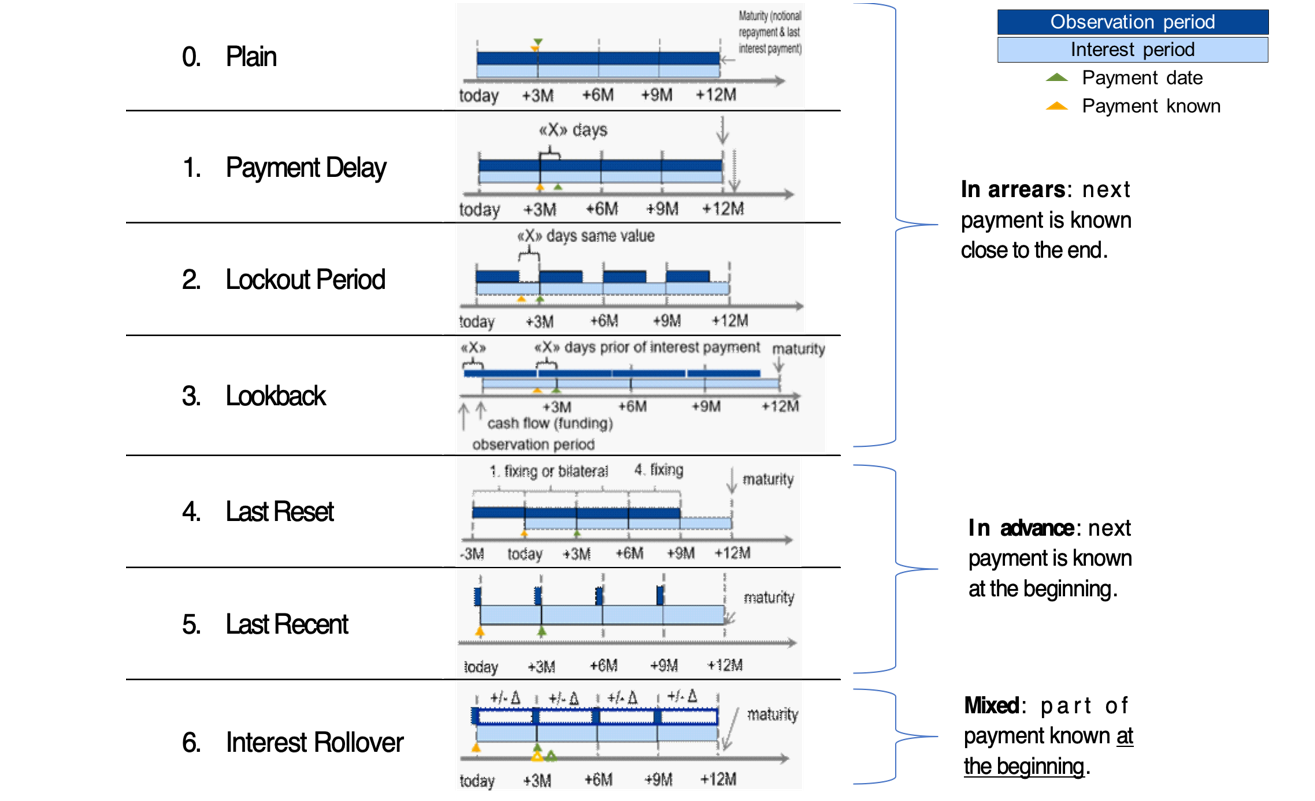
Figure 1: Overview of alternative techniques for calculating compounded SARON. Source: Financial Stability Board (2019).
0) Plain (in arrears): The observation period is identical to the interest period. The notional is paid at the start of the period and repaid on the last day of the contract period together with the last interest payment. Moreover, a Plain (in arrears) structure reflects the movement in interest rates over the full interest period and the payment is made on the day that it would naturally be due. On the other hand, given publication timing for most RFRs (T+1), the requiring payment is on the same day (T+1) that the final payment amount is known (T+1). An exception is SARON, as SARON is published one business day (T+0) before the overnight loan is repaid (T+1).
Example: the 1-month compounded SARON based on the Plain technique is like the example explained in the previous article, but has a different start date (1 February 2019). The resulting 1-month compounded SARON is equal to -0.7340% and it is known one day before the payment date (i.e. known on 28 February 2019).
1) Payment Delay (in arrears): Interest rate payments are delayed by X days after the end of an interest period. The idea is to provide more time for operational cash flow management. If X is set to 2 days, the cash flow of the loan matches the cash flow of most OIS swaps. This allows perfect hedging of the loan. On the other hand, the payment in the last period is due after the payback of the notional, which leads to a mismatch of cash flows and a potential increase in credit risk.
Example: the 1-month compounded SARON is equal to -0.7340% and like the one calculated using the Plain (in arrears) technique. The only difference is that the payment date shifts by X days, from 1 March 2019 to e.g. 4 March 2019. In this case X is equal to 3 days.
2) Lockout Period (in arrears): The RFR is no longer updated, i.e. frozen, for X days prior to the end of an interest rate period (lockout period). During this period, the RFR on the day prior to the start of the lockout is applied for the remaining days of the interest period. This technique is used for SOFR-based Floating Rate Notes (FRNs), where a lockout period of 2-5 days is mostly used in SOFR FRNs. Nevertheless, the calculation of the interest rate might be considered less transparent for clients and more complex for product providers to be implemented. It also results in interest rate risk that is difficult to hedge due to potential changes in the RFR during the lockout period. The longer the lockout period, the more difficult interest rate risk can be hedged during the lockout period.
Example: the 1-month compounded SARON with a lockout period equal to 3 days (i.e. X equals 3 days) is equal to -0.7337% and known 3 days in advance of the payment date.
3) Lookback (in arrears): The observation period for the interest rate calculation starts and ends X days prior to the interest period. Therefore, the interest payments can be calculated prior to the end of the interest period. This technique is predominately used for SONIA-based FRNs with a delay period of X equal to 5 days. An increase in interest rate risk due to changes in yield curve is observed over the lifetime of the product. This is expected to make it more difficult to hedge interest rate risk.
Example: assuming X is equal to 3 days, the 1-month compounded SARON would start in advance, on January 29, 2019 (i.e. today minus 3 days). This technique results in a compounded 1-month SARON equal to -0.7335%, known on 25 February 2019 and payable on 1 March 2019.
4) Last Reset (in advance): Interest payments are based on compounded RFR of the previous period. It is possible to ensure that the present value is equivalent to the Plain (in arrears) case, thanks to a constant mark-up added to the compounded RFR. The mark-up compensates the effects of the period shift over the full life of the product and can be priced by the OIS curve. In case of a decreasing yield curve, the mark-up would be negative. With this technique, the product is more complex, but the interest payments are known at the start of the interest period, as a LIBOR-based product. For this reason, the mark-up can be perceived as the price that a borrower is willing to pay due to the preference to know the next payment in advance.
Example: the interest rate payment on 1 March 2019 is already known at the start date and equal to -0.7328% (without mark-up).
5) Last Recent (in advance): A single RFR or a compounded RFR for a short number of days (e.g. 5 days) is applied for the entire interest period. Given the short observation period, the interest payment is already known in advance at the start of each interest period and due on the last day of that period. As a consequence, the volatility of a single RFR is higher than a compounded RFR. Therefore, interest rate risk cannot be properly hedged with currently existing derivatives instruments.
Example: a 5-day average is used to calculate the compounded SARON in advance. On the start date, the compounded SARON is equal to -0.7339% (known in advance) that will be paid on 1 March 2020.
6) Interest Rollover (hybrid): This technique combines a first payment (installment payment) known at the beginning of the interest rate period with an adjustment payment known at the end of the period. Like Last Recent (in advance), a single RFR or a compounded RFR for a short number of days is fixed for the whole interest period (installment payment known at the beginning). At the end of the period, an adjustment payment is calculated from the differential between the installment payment and the compounded RFR realized during the interest period. This adjustment payment is paid (by either party) at the end of the interest period (or a few days later) or rolled over into the payment for the next interest period. In short, part of the interest payment is known already at the start of the period. Early termination of contracts becomes more complex and a compensation mechanism is needed.
Example: similar to Last Recent (in advance), a 5-day compounded SARON can be considered as installment payment before the starting date. On the starting date, the 5-day compounded SARON rate is equal to -0.7339% and is known to be paid on 1 March 2019 (payment date). On the payment date, an adjustment payment is calculated as the delta between the realized 1-month compounded SARON, equal to -0.7340% based on Plain (in arrears), and -0.7339%.
There is a trade-off between knowing the cash flows in advance and the desire for a payment structure that is fully hedgeable against realized interest rate risk. Instruments in the derivatives market currently use ‘in arrears’ payment structures. As a result, the more the option used for a cash product deviates from ‘in arrears’, the less efficient the hedge for such a cash product will be. In order to use one or more of these options for cash products, operational cash management (infrastructure) systems need to be updated. For more details about the calculation of the compounded SARON using the alternative techniques, please refer to Table 1 and Table 2 in the Appendix I. The compounding formula used in the calculation is explained in the previous article.
Overall, market participants are recommended to consider and assess all the options above. Moreover, the financial institutions should individually define action plans with respect to their own product strategies.
Conclusions
The transition from IBOR to alternative reference rates affects all financial institutions from a wide operational perspective, including how products are created. Existing LIBOR-based cash products need to be replaced with SARON-based products as the mortgages contract. In the next installment, IBOR Reform in Switzerland – Part III, the latest information from the Swiss National Working Group (NWG) and market developments on the compounded SARON will be explained in more detail.
Contact
For more information about the challenges and latest developments on SARON, please contact Martijn Wycisk or Davide Mastromarco of Zanders’ Swiss office: +41 44 577 70 10.
The other articles on this subject:
Transition from CHF LIBOR to SARON, IBOR Reform in Switzerland, Part I
Compounded SARON and Swiss Market Development, IBOR Reform in Switzerland, Part III
Fallback provisions as safety net, IBOR Reform in Switzerland, Part IV
References
- Mastromarco, D. Transition from CHF LIBOR to SARON, IBOR Reform in Switzerland – Part I. February 2020.
- National Working Group on Swiss Franc Reference Rates. Discussion paper on SARON Floating Rate Notes. July 2019.
- National Working Group on Swiss Franc Reference Rates. Executive summary of the 12 November 2019 meeting of the National Working Group on Swiss Franc Reference Rates. Press release November 2019.
- National Working Group on Swiss Franc Reference Rates. Starter pack: LIBOR transition in Switzerland. December 2019.
- Financial Stability Board (FSB). Overnight Risk-Free Rates: A User’s Guide. June 2019.
- ISDA. Supplement number 60 to the 2006 ISDA Definitions. October 2019.
- ISDA. Interbank Offered Rate (IBOR) Fallbacks for 2006 ISDA Definitions. December 2019.
- National Working Group on Swiss Franc Reference Rates. Executive summary of the 7 May 2020 meeting of the National Working Group on Swiss Franc Reference Rates. Press release May 2020

Martijn Habing, head of Model Risk Management (MoRM) at ABN AMRO bank, spoke at the Zanders Risk Management Seminar about the extent to which a model can predict the impact of an event.
The MoRM division of ABN AMRO comprises around 45 people. What are the crucial conditions to run the department efficiently?
Habing: “Since the beginning of 2019, we have been divided into teams with clear responsibilities, enabling us to work more efficiently as a model risk management component. Previously, all questions from the ECB or other regulators were taken care of by the experts of credit risk, but now we have a separate team ready to focus on all non-quantitative matters. This reduces the workload on the experts who really need to deal with the mathematical models. The second thing we have done is to make a stronger distinction between the existing models and the new projects that we need to run. Major projects include the Definition of default and the introduction of IFRS 9. In the past, these kinds of projects were carried out by people who actually had to do the credit models. By having separate teams for this, we can scale more easily to the new projects – that works well.”What exactly is the definition of a model within your department? Are they only risk models, or are hedge accounting or pricing models in scope too?
“We aim to identify the widest range of models as possible, both in size and type. From an administrative point of view, we can easily do 600 to 700 models. But with such a number, we can't validate them all in the same degree of depth. We therefore try to get everything in picture, but this varies per model what we look at.”
To what extent does the business determine whether a validation model is presented?
“We want to have all models in view. Then the question is: how do you get a complete overview? How do you know what models there are if you don't see them all? We try to set this up in two ways. On the one hand, we do this by connecting to the change risk assessment process. We have an operational risk department that looks at the entire bank in cycles of approximately three years. We work with operational risk and explain to them what they need to look out for, what ‘a model’ is according to us and what risks it can contain. On the other hand, we take a top-down approach, setting the model owner at the highest possible level. For example, the director of mortgages must confirm for all processes in his business that the models have been well developed, and the documentation is in order and validated. So, we're trying to get a view on that from the top of the organization. We do have the vast majority of all models in the picture.”
Does this ever lead to discussion?
“Yes, that definitely happens. In the bank's policy, we’ve explained that we make the final judgment on whether something is a model. If we believe that a risk is being taken with a model, we indicate that something needs to be changed.”
Some of the models will likely be implemented through vendor systems. How do you deal with that in terms of validation?
“The regulations are clear about this: as a bank, you need to fully understand all your models. We have developed a vast majority of the models internally. In addition, we have market systems for which large platforms have been created by external parties. So, we are certainly also looking at these vendor systems, but they require a different approach. With these models you look at how you parametrize – which test should be done with it exactly? The control capabilities of these systems are very different. We're therefore looking at them, but they have other points of interest. For example, we perform shadow calculations to validate the results.”
How do you include the more qualitative elements in the validation of a risk model?
“There are models that include a large component from an expert who makes a certain assessment of his expertise based on one or more assumptions. That input comes from the business itself; we don't have it in the models and we can't control it mathematically. At MoRM, we try to capture which assumptions have been made by which experts. Since there is more risk in this, we are making more demands on the process by which the assumptions are made. In addition, the model outcome is generally input for the bank's decision. So, when the model concludes something, the risk associated with the assumptions will always be considered and assessed in a meeting to decide what we actually do as a bank. But there is still a risk in that.”
How do you ensure that the output from models is applied correctly?
“We try to overcome this by the obligation to include the use of the model in the documentation. For example, we have a model for IFRS 9 where we have to indicate that we also use it for stress testing. We know the internal route of the model in the decision-making of the bank. And that's a dynamic process; there are models that are developed and used for other purposes three years later. Validation is therefore much more than a mathematical exercise to see how the numbers fall apart.”
Typically, the approach is to develop first, then validate. Not every model will get a ‘validation stamp’. This can mean that a model is rejected after a large amount of work has been done. How can you prevent this?
“That is indeed a concrete problem. There are cases where a lot of work has been put into the development of a new model that was rejected at the last minute. That's a shame as a company. On the one hand, as a validation department, you have to remain independent. On the other hand, you have to be able to work efficiently in a chain. These points can be contradictory, so we try to live up to both by looking at the assumptions of modeling at an early stage. In our Model Life Cycle we have described that when developing models, the modeler or owner has to report to the committee that determines whether something can or can’t. They study both the technical and the business side. Validation can therefore play a purer role in determining whether or not something is technically good.”
To be able to better determine the impact of risks, models are becoming increasingly complex. Machine learning seems to be a solution to manage this, to what extent can it?
“As a human being, we can’t judge datasets of a certain size – you then need statistical models and summaries. We talk a lot about machine learning and its regulatory requirements, particularly with our operational risk department. We then also look at situations in which the algorithm decides. The requirements are clearly formulated, but implementation is more difficult – after all, a decision must always be explainable. So, in the end it is people who make the decisions and therefore control the buttons.”
To what extent does the use of machine learning models lead to validation issues?
“Seventy to eighty percent of what we model and validate within the bank is bound by regulation – you can't apply machine learning to that. The kind of machine learning that is emerging now is much more on the business side – how do you find better customers, how do you get cross-selling? You need a framework for that; if you have a new machine learning model, what risks do you see in it and what can you do about it? How do you make sure your model follows the rules? For example, there is a rule that you can't refuse mortgages based on someone's zip code, and in the traditional models that’s well in sight. However, with machine learning, you don't really see what's going on ‘under the hood’. That's a new risk type that we need to include in our frameworks. Another application is that we use our own machine learning models as challenger models for those we get delivered from modeling. This way we can see whether it results in the same or other drivers, or we get more information from the data than the modelers can extract.”
How important is documentation in this?
“Very important. From a validation point of view, it’s always action point number one for all models. It’s part of the checklist, even before a model can be validated by us at all. We have to check on it and be strict about it. But particularly with the bigger models and lending, the usefulness and need for documentation is permeated.”
Finally, what makes it so much fun to work in the field of model risk management?
“The role of data and models in the financial industry is increasing. It's not always rewarding; we need to point out where things go wrong – in that sense we are the dentist of the company. There is a risk that we’re driven too much by statistics and data. That's why we challenge our people to talk to the business and to think strategically. At the same time, many risks are still managed insufficiently – it requires more structure than we have now. For model risk management, I have a clear idea of what we need to do to make it stronger in the future. And that's a great challenge.”

In 2014, with its Think Forward strategy, ING set the goal to further standardize and streamline its organization. At the time, changes in international regulations were also in full swing. But what did all this mean for risk management at the bank? We asked ING’s Constant Thoolen and Gilbert van Iersel.
According to Constant Thoolen, global head of financial risk at ING, the Accelerating Think Forward strategy, an updated version of the Think Forward strategy that they just call ATF, comprises several different elements.
"Standardization is a very important one. And from standardization comes scalability and comparability. To facilitate this standardization within the financial risk management team, and thus achieve the required level of efficiency, as a bank we first had to make substantial investments so we could reap greater cost savings further down the road."
And how exactly did ING translate this into financial risk management?
Thoolen: "Obviously, there are different facets to that risk, which permeates through all business lines. The interest rate risk in the banking book, or IRRBB, is a very important part of this. Alongside the interest rate risk in trading activities, the IRRBB represents an important risk for all business lines. Given the importance of this type of risk, and the changing regulatory complexion, we decided to start up an internal IRRBB program."
So the challenge facing the bank was how to develop a consistent framework in benchmarking and reporting the interest rate risk?
"The ATF strategy has set requirements for the consistency and standardization of tooling," explains Gilbert van Iersel, head of financial risk analysis. "On the one hand, our in-house QRM program ties in with this. We are currently rolling out a central system for our ALM activities, such as analyses and risk measurements—not only from a risk perspective but from a finance one too. Within the context of the IRRBB program, we also started to apply this level of standardization and consistency throughout the risk-management framework and the policy around it. We’re doing so by tackling standardization in terms of definitions, such as: what do we understand by interest rate risk, and what do benchmarks like earnings-at-risk or NII-at-risk actually mean? It’s all about how we measure and what assumptions we should make."
What role did international regulations play in all this?
Van Iersel: "An important one. The whole thing was strengthened by new IRRBB guidelines published by the EBA in 2015. It reconciled the ATF strategy with external guidelines, which prompted us to start up the IRRBB program."
So regulations served as a catalyst?
Thoolen: "Yes indeed. But in addition to serving as a foothold, the regulations, along with many changes and additional requirements in this area, also posed a challenge. Above all, it remains in a state of flux, thanks to Basel, the EBA, and supervision by the ECB. On the one hand, it’s true that we had expected the changes, because IRRBB discussions had been going on for some time. On the other hand, developments in the regulatory landscape surrounding IRRBB followed one another quite quickly. This is also different from the implementation of Basel II or III, which typically require a preparation and phasing-in period of a few years. That doesn’t apply here because we have to quickly comply with the new guidelines."
Did the European regulations help deliver the standardization that ING sought as an international bank?
Thoolen: "The shift from local to European supervision probably increased our need for standardization and consistency. We had national supervisors in the relevant countries, each supervising in their own way, with their own requirements and methodologies. The ECB checked out all these methodologies and created best practices on what they found. Now we have to deal with regulations that take in all Eurozone countries, which are also countries in which ING is active. Consequently, we are perfectly capable of making comparisons between the implementation of the ALM policy in the different countries. Above all, the associated risks are high on the agenda of policymakers and supervisors."
Van Iersel: "We have also used these standards in setting up a central treasury organization, for example, which is also complementary to the consistency and standardization process."
Thoolen: "But we’d already set the further integration of the various business units in motion, before the new regulations came into force. What’s more, we still have to deal with local legislation in the countries in which we operate outside Europe, such as Australia, Singapore, and the US. Our ideal world would be one in which we have one standard for our calculations everywhere."
What changed in the bank’s risk appetite as a result of this changing environment and the new strategy?
Van Iersel: "Based on newly defined benchmarks, we’ve redefined and shaped our risk appetite as a component part of the strategic program. In the risk appetite process we’ve clarified the difference between how ING wants to manage the IRRBB internally and how the regulator views the type of risk. As a bank, you have to comply with the so-called standard outlier test when it comes to the IRRBB. The benchmark commonly employed for this is the economic value of equity, which is value-based. Within the IRRBB, you can look at the interest rate risk from a value or an income perspective. Both are important, but they occasionally work against one another too. As a bank, we’ve made a choice between them. For us, a constant stream of income was the most important benchmark in defining our interest rate risk strategy, because that’s what is translated to the bottom line of the results that we post. Alongside our internal decision to focus more closely on income and stabilize it, the regulator opted to take a mainly value-based approach. We have explicitly incorporated this distinction in our risk appetite statements. It’s all based on our new strategy; in other words, what we are striving for as a bank and what will be the repercussions for our interest rate risk management. It’s from there that we define the different risk benchmarks."
Which other types of risk does the bank look at and how do they relate to the interest rate risk?
Van Iersel: “From the financial risk perspective, you also have to take into account aspects like credit spreads, changes in the creditworthiness of counterparties, as well as market-related risks in share prices and foreign exchange rates. Given that all these collectively influence our profitability and solvency position, they are also reflected in the Core Tier I ratio. There is a clear link to be seen there between the risk appetite for IRRBB and the overall risk appetite that we as a bank have defined. IRRBB is a component part of the whole, so there’s a certain amount of interaction between them to be considered; in other words, how does the interest rate risk measure up to the credit risk? On top of that, you have to decide where to deploy your valuable capacity. All this has been made clearer in this program.”
Does this mean that every change in the market can be accommodated by adjusting the risk appetite?
Thoolen: “Changing behavior can indeed influence risks and change the risk appetite, although not necessarily. But it can certainly lead to a different use of risk. Moreover, IFRS 9 has changed the accounting standards. Because the Core Tier 1 ratio is based on the accounting standard, these IFRS 9 changes determine the available capital too. If IFRS 9 changes the playing field, it also exerts an influence on certain risk benchmarks.”
In addition to setting up a consistent framework, the standardization of the models used by the different parts of ING was also important. How does ING approach the selection and development of these models?
Thoolen: “With this in mind, we’ve set up a structure with the various business units that we collaborate with from a financial risk perspective. We pay close attention to whether a model is applicable in the environment in which it’s used. In other words, is it a good fit with what’s happening in the market, does it cover all the risks as you see them, and does it have the necessary harmony with the ALM system? In this way, we want to establish optimum modeling for savings or the repayment risk of mortgages, for example.”
But does that also work for an international bank with substantial portfolios in very different countries?
Thoolen: “While there is model standardization, there is no market standardization. Different countries have their own product combinations and, outside the context of IRRBB, have to comply with regulations that differ from other countries. A savings product in the Netherlands will differ from a savings product in Belgium, for example. It’s difficult to define a one-size-fits-all model because the working of one market can be much more specific than another—particularly when it comes to regulations governing retail and wholesale. This sometimes makes standardization more difficult to apply. The challenge lies in the fact that every country and every market is specific, and the differences have to be reconciled in the model.”
Van Iersel: “The model was designed to measure risks as well as possible and to support the business to make good decisions. Having a consistent risk appetite framework can also make certain differences between countries or activities more visible. In Australia, for example, many more floating-rate mortgages are sold than here in the Netherlands, and this alters the sensitivity of the bank’s net interest income when the interest rate changes. Risk appetite statements must facilitate such differences.”
To what extent does the use of machine learning models lead to validation issues?
“Seventy to eighty percent of what we model and validate within the bank is bound by regulation – you can't apply machine learning to that. The kind of machine learning that is emerging now is much more on the business side – how do you find better customers, how do you get cross-selling? You need a framework for that; if you have a new machine learning model, what risks do you see in it and what can you do about it? How do you make sure your model follows the rules? For example, there is a rule that you can't refuse mortgages based on someone's zip code, and in the traditional models that’s well in sight. However, with machine learning, you don't really see what's going on ‘under the hood’. That's a new risk type that we need to include in our frameworks. Another application is that we use our own machine learning models as challenger models for those we get delivered from modeling. This way we can see whether it results in the same or other drivers, or we get more information from the data than the modelers can extract.”
Thoolen: “But opting for a single ALM system imposes this model standardization on you and ensures that, once it’s integrated, it will immediately comply with many conditions. The process is still ongoing, but it’s a good fit with the standardization and consistency that we’re aiming for.”
In conjunction with the changing regulatory environment, the Accelerating Think Forward Strategy formed the backdrop for a major collaboration with Zanders: the IRRBB project. In the context of this project, Zanders researched the extent to which the bank’s interest rate risk framework complied with the changing regulations. The framework also assessed ING’s new interest rate risk benchmarks and best practices. Based on the choices made by the bank, Zanders helped improve and implement the new framework and standardized models in a central risk management system.

With the advance of the current low interest rate environment and increased regulatory requirements, modeling mortgages for valuation purposes is more complex. Additionally, the applicable valuation method depends on the purpose of the valuation.
The most common valuation method for mortgage funds is known as the ‘fair value’ method, consisting of two building blocks: the cash flows and a discount curve. The first prerequisite to apply the fair value method is to determine future cash flows, based on the contractual components and behavioral modeling. The other prerequisite is to derive the appropriate rate for discounting via a top-down or bottom-up approach.
Two building blocks
The appropriate approach and level of complexity in the mortgage valuation depend on the underlying purpose. Examples of valuation purposes are: regulatory, accounting, risk or sales of the mortgage portfolio. For example BCBS, IRRBB, Solvency, IFRS and the EBA ask for (specific) valuation methods of mortgages. The two building blocks for a ‘fair value’ calculation of mortgages are expected cash flows and a discount curve.
The market value is the sum of the expected cash flows at the moment of valuation, which are derived by discounting future expected cash flows with an appropriate curve. For both building block models, choices have to be made resulting in a tradeoff between the accuracy level and the computational effort.
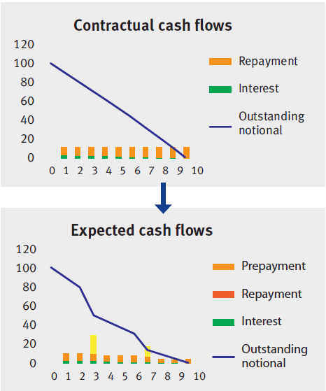
Figure 1: Constructing the expected cash flows from the contractual cash flows for a loan with an annuity repayment type.
Cash flow schedule
The contractual cash flows are projected cash flows, including repayments. These can be derived based on the contractually agreed loan components, such as the interest rate, the contractual maturity and the redemption type.
The three most commonly used redemption types in the mortgage market are:
- Bullet: interest only payments, no contractual repayment cash flows except at maturity
- Linear: interest (decreasing monthly) and constant contractual repayment cash flows
- Annuity: fixed cash flows, consisting of an interest and contractual repayment part
However, the expected cash flows will most likely differ from this contractually agreed pattern due to additional prepayments. Especially in the current low interest rate environment, borrowers frequently make prepayments on top of the scheduled repayments.
Figure 1 shows how to calculate an expected cash flow schedule by adding the prepayment cash flows to the contractual cash flow. There are two methods to derive : client behavior dependent on interest rates and client behavior independent of interest rates. The independent method uses an historical analysis, indicating a backward looking element. This historical analysis can include a dependency on certain contract characteristics.
On the other hand, the interest rate dependent behavior is forward looking and depends on the expected level of the interest rates. Monte Carlow simulations can model interest dependent behavior.
Another important factor in client behavior are penalties paid in case of a prepayment above a contractually agreed threshold. These costs are country and product specific. In Italy, for example, these extra costs do not exist, which could currently result in high prepayments rates.
Discount curve
The curve used for cash flow discounting is always a zero curve. The zero curve is constructed from observed interest rates which are mapped on zero-coupon bonds to maturities across time. There are three approaches to derive the rates of this discount curve: the top down-approach, the bottom-up approach or the negotiation approach. The first two methods are the most relevant and common.
In theory, an all-in discount curve consists of a riskfree rate and several spread components. The ‘base’ interest curve concerns the risk-free interest rate term structure in the market at the valuation date with the applicable currency and interest fixing frequency (or use ccy- and basis-spreads). The spreads included depend on the purpose of the valuation. For a fair value calculation, the following spreads are added: liquidity spread, credit spread, operational cost, option cost, cost of capital and profit margin. An example of spreads included for other valuation purposes are offerings costs and origination fee.
Top-down versus Bottom-up
The chosen calculation approach depends on the available data, the ability to determine spread components, preferences and the purpose of the valuation.
A top-down method derives the applied rates of the discount curve from all-in mortgage rates on a portfolio level. Different rates should be used to construct a discount curve per mortgage type and LTV level, and should take into account the national guaranteed amount (NHG in the Netherlands). Subtract all-in mortgage rates spreads that should not part of the discount curve, such as the offering costs. Use this top-down approach when limited knowledge or tools are available to derive all the individual spread components. The all-in rates can be obtained from the following sources: mortgage rates in the market, own mortgage rates or by designing a mortgage pricing model.
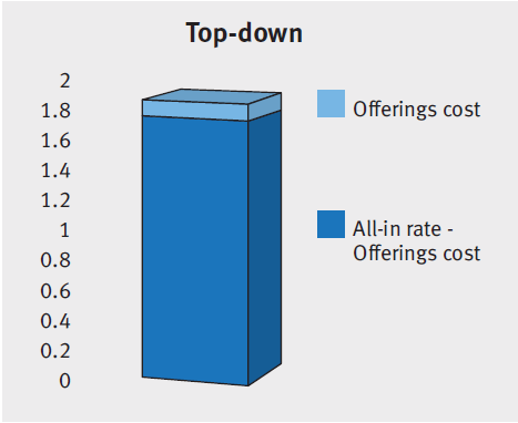
Figure 2
The bottom-up approach constructs the applied discount curve by adding all applicable spreads on top of the zero curve at a contract level. This method requires that several spread components can be calculated separately. The top-down approach is quicker, but less precise than the bottom-up approach, which is more accurate but also computationally heavy. Additionally, the bottom-up method is only possible if the appropriate spreads are known or can be derived. One example of a derivation of a spread component is credit spreads determined from expected losses based on an historical analysis and current market conditions.
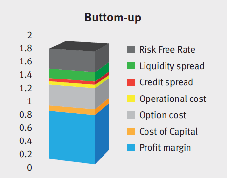
In short
A fair value calculation performed by a discounted cash flow method consists of two building blocks: the expected cash flows and a discount curve. This requires several model choices before calculating a fair value of a mortgage (portfolio).
The expected cash flow model is based on the contractual cash flows and any additional prepayments. The mortgage prepayments can be modeled by assuming interest dependent or interest independent client behavior.
To construct the discount curve, the relevant spreads should be added to the risk-free curve. The decision for a top-down or bottom-up approach depends on the available data, the ability to determine spread components, preferences and the purpose of the valuation.
These important choices do not only apply for fair value calculations but are applicable for many other mortgage valuation purposes.
Zanders Valuation Desk
Independent, high quality, market practice and accounting standard proof are the main drivers of our Valuation Desk. For example, we ensure a high quality and professionalism with a strict, complete and automated check on the market data from our market data provider on a daily basis. Furthermore, we have increased our independence by implementing the F3 solution from FINCAD in our current valuation models. This permits us to value a larger range of financial instruments with a high level of quality, accuracy and wider complexity.
For more information or questions concerning valuation issues, please contact Pierre Wernert: [email protected].

On 18 May 2017, the International Accounting Standard Board (IASB) issued the new IFRS 17 standards. The development of these standards has been a long and thorough process with the aim of providing a single global comprehensive accounting standard for insurance contracts.
The new standards will have a significant impact on the measurement and presentation of insurance contracts in the financial statements and require significant operational changes. This article takes a closer look at the new standards, and illustrates the impact with a case study.
The standard model, as defined by IFRS 17, of measuring the value of insurance contracts is the ‘building blocks approach’. In this approach, the value of the contract is measured as the sum of the following components:
- Block 1: Sum of the future cash flows that relate directly to the fulfilment of the contractual obligations.
- Block 2: Time value of the future cash flows. The discount rates used to determine the time value reflect the characteristics of the insurance contract.
- Block 3: Risk adjustment, representing the compensation that the insurer requires for bearing the uncertainty in the amount and timing of the cash flows.
- Block 4: Contractual service margin (CSM), representing the amount available for overhead and profit on the insurance contract. The purpose of the CSM is to prevent a gain at initiation of the contract.
Risk adjustment vs risk margin
IFRS 17 does not provide full guidance on how the risk adjustment should be calculated. In theory, the compensation required by the insurer for bearing the risk of the contract would be equal to the cost of the needed capital. As most insurers within the IFRS jurisdiction capitalize based on Solvency II (SII) standards, it is likely that they will leverage on their past experience. In fact, there are many similarities between the risk adjustment and the SII risk margin.
The risk margin represents the compensation required for non-hedgeable risks by a third party that would take over the insurance liabilities. However, in practice, this is calculated using the capital models of the insurer itself. Therefore, it seems likely that the risk margin and risk adjustment will align. Differences can be expected though. For example, SII allows insurers to include operational risk in the risk margin, while this is not allowed under IFRS 17.
Liability adequacy test
Determining the impact of IFRS 17 is not straightforward: the current IFRS accounting standard leaves a lot of flexibility to determine the reserve value for insurance liabilities (one of the reasons for introducing IFRS 17). The reserve value reported under current IFRS is usually grandfathered from earlier accounting standards, such as Dutch GAAP. In general, these reserves can be defined as the present value of future benefits, where the technical interest rate and the assumptions for mortality are locked-in at pricing.
However, insurers are required to perform liability adequacy testing (LAT), where they compare the reserve values with the future cash flows calculated with ‘market consistent’ assumptions. As part of the market consistent valuation, insurers are allowed to include a compensation for bearing risk, such as the risk adjustment. Therefore, the biggest impact on the reserve value is expected from the introduction of the CSM.
The IASB has defined a hierarchy for the approach to measure the CSM at transition date. The preferred method is the ‘full retrospective application’. Under this approach, the insurer is required to measure the insurance contract as if the standard had always applied. Hence, the value of the insurance contract needs to be determined at the date of initial recognition and consecutive changes need to be determined all the way to transition date. This process is outlined in the following case study.
A case study
The impact of the new IFRS standards is analyzed for the following policy:
- The policy covers the risk that a mortgage owner deceases before the maturity of the loan. If this event occurs, the policy pays the remaining notional of the loan.
- The mortgage is issued on 31 December 2015 and has an initial notional value of € 200,000 that is amortized in 20 years. The interest percentage is set at 3 per cent.
- The policy pays an annual premium of € 150. The annual estimated costs of the policy are equal to 10 per cent of the premium.
In the case of this policy, an insurer needs to capitalize for the risk that the policy holder’s life expectancy decreases and the risk that expenses will increase (e.g. due to higher than expected inflation). We assume that the insurer applies the SII standard formula, where the total capital is the sum of the capital for the individual risk types, based on 99.5 per cent VaR approach, taking diversification into account.
The cost of capital would then be calculated as follows:
- Capital for mortality risk is based on an increase of 15 per cent of the mortality rates.
- Capital for expense risk is based on an increase of 10 per cent in expense amount combined with an increase of 1 per cent in the inflation.
- The diversification between these risk types is assumed to be 25 per cent.
- Future capital levels are assumed to be equal to the current capital levels, scaled for the decrease in outstanding policies and insurance coverage.
- The cost-of-capital rate equals 6 per cent.
At initiation (i.e. 2015 Q4), the value of the contract under the new standards equals the sum of:
- Block 1: € 482
- Block 2: minus € 81
- Block 3: minus € 147
- Block 4: minus € 254
Consecutive changes
The insurer will measure the sum of blocks 1, 2 and 3 (which we refer to as the fulfilment cash flows) and the remaining amount of the CSM at each reporting date. The amounts typically change over time, in particular when expectations about future mortality and interest rates are updated. We distinguish four different factors that will lead to a change in the building blocks:
Step 1. Time effect
Over time, both the fulfilment cash flows and the CSM are fully amortized. The amortization profile of both components can be different, leading to a difference in the reserve value.
Step 2. Realized mortality is lower than expected
In our case study, the realized mortality is about 10 per cent lower than expected. This difference is recognized in P&L, leading to a higher profit in the first year. The effect on the fulfilment cash flows and CSM is limited. Consequently, the reserve value will remain roughly the same.
Step 3. Update of mortality assumptions
Updates of the mortality assumptions affect the fulfilment cash flows, which is simultaneously recognized in the CSM. The offset between the fulfilment cash flows and the CSM will lead to a very limited impact on the reserve value. In this case study, the update of the life table results in higher expected mortality and increased future cash outflows.
Step 4. Decrease in interest rates
Updates of the interest rate curve result in a change in the fulfilment cash flows. This change is not offset in the CSM, but is recognized in the other comprehensive income. Therefore a decrease in the discount curve will result in a significant change in the insurance liability. Our case study assumes a decrease in interest rates from 2 per cent to 1 per cent. As a result, the fulfilment cash flows increase, which is immediately reflected by an increase in the reserve value.
The impact of each step on the reserve value and underlying blocks is illustrated below.
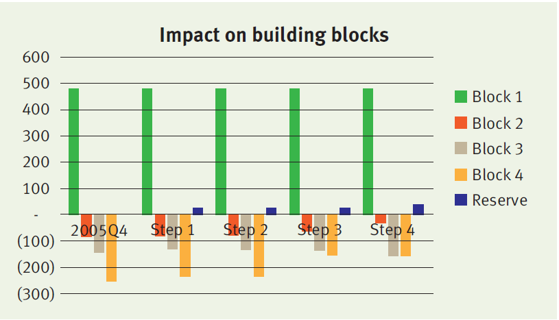
Onwards
The policy will evolve over time as expected, meaning that mortality will be realized as expected and discount rates do not change anymore. The reserve value and P&L over time will evolve as illustrated below.
The profit gradually decreases over time in line with the insurance coverage (i.e. outstanding notional of the mortgage). The relatively high profit in 2016 is (mainly) the result of the realized mortality that was lower than expected (step 2 described above).
As described before, under the full retrospective application, the insurer would be required to go all the way back to the initial recognition to measure the CSM and all consecutive changes. This would require insurers to deep-dive back into their policy administration systems. This has been acknowledged by the IASB by allowing insurers to implement the standards three years after final publication. Insurers will have to undertake a huge amount of operational effort and have already started with their impact analyses. In particular, the risk adjustment seems a challenging topic that requires an understanding of the capital models of the insurer.
Zanders can support in these qualitative analyses and can rely on its past experience with the implementation of Solvency II.