

How financial institutions can move from siloed valuation models to a cohesive framework that enhances transparency and operational efficiency.
The Proliferation of Valuation Models
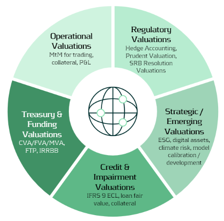
Valuation lies at the heart of financial institutions — informing decisions in trading, risk management, collateral management, accounting, and financial reporting. Yet across many banks, these valuations are performed in fragmented silos for different purposes, using different models, data sources, and systems. In addition to these core applications, valuations also support a broader range of activities, including treasury, regulatory reporting, and emerging domains such as ESG and digital assets.
As illustrated in the Valuation Map (Figure 1), we observe that in many cases different departments conduct their own valuations, often for their own distinct purposes and using distinct valuation processes. Survey evidence shows that finance and FP&A teams devote roughly 65% of their time to data gathering, cleaning, and reconciliation, leaving only about 35% for value-adding analysis1.
The Cost of Fragmentation
Fragmented valuation architectures translate directly into higher costs and operational drag. In practice, three effects are most pronounced:
- High data vendor spend – market-data pricing surveys found that some firms were paying “many multiples” more than peers for similar products and use cases, reflecting redundant sourcing and poor usage visibility2.
- Model proliferation – large banks often operate with hundreds to thousands of models across the enterprise, creating overlap in purpose and increasing governance, maintenance, and compute costs3.
- Inconsistent and time-consuming valuations – disparate models and data feeds lead to unclear ownership of valuation “truth” and significant manual reconciliation between accounting, risk, and front-office views.
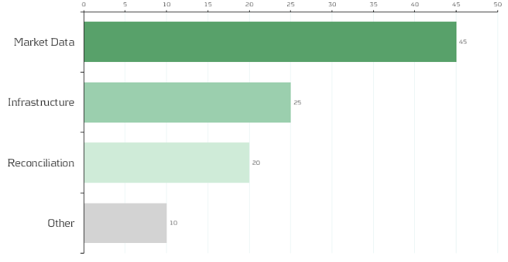
Although no public benchmark precisely mirrors our allocation, multiple industry surveys converge on the same conclusion: market data represents a dominant share of valuation costs, and fragmented reconciliation processes account for a significant portion of non-value-adding effort. Figure 2 therefore shows an indicative distribution — 45% market data, 25% infrastructure, 20% reconciliation, 10% other — to convey the relative scale of each component. Institutions will vary in mix, yet the implication is consistent: rationalizing data sourcing and automating reconciliation are among the highest-impact levers for reducing total valuation cost.
Strategic Imperative: Centralizing and Standardizing Valuation
Banks can unlock substantial efficiency gains by centralizing valuation logic and governing data flows. Similar to how treasury departments manage liquidity, banks should treat valuation processes as coordinated enterprise capabilities rather than fragmented operational activities.
Key levers include:
1-Valuation as a Service (VaaS):
Establish a centralized valuation engine providing consistent pricing APIs for all functions (risk, finance, collateral, etc.).
2-Unified Market Data Platform:
Integrate vendor feeds into a single validated golden source with standardized identifiers and governance.
3-Model Consolidation and Validation:
Maintain one approved model per product type with clear ownership and lifecycle management.
4- Process Automation:
Automate reconciliation between accounting and risk views via shared data lineage and valuation transparency.
5- Cost Transparency:
Track valuation and data usage per business unit to encourage accountability and optimization.
Together, these measures reduce duplication, accelerate reporting cycles, and improve consistency across valuation outcomes.
Building the Foundation
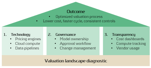
An optimized valuation operating model rests on three mutually reinforcing foundations:
- Technology: Scalable pricing engines, cloud compute elasticity, and efficient data pipelines.
- Governance: Clear model ownership, approval, and change management across risk and finance.
- Transparency: Dashboards tracking valuation cost, compute time, and data provider usage.
A practical first step: Zanders can perform a valuation landscape diagnostic, mapping all valuation types, systems, and data sources. Such analysis typically reveals 10–20% potential overlap and quick wins in data consolidation4.
Conclusion: Elevating Valuation Processes to an Enterprise Capability
In today’s environment of cost pressure and regulatory scrutiny, optimizing valuation processes is not only about efficiency—it is about strengthening consistency, transparency, and trust across the organization. Institutions that unify valuation workflows, data, and governance are better positioned to:
- Reduce operational costs and reconciliation workloads.
- Rationalize compute power – costs of running multiple models unnecessarily.
- Strengthen governance and auditability.
- Accelerate model deployment and reporting cycles.
- Enable transparent, sustainable, and data-driven decision-making.
At Zanders, we design and implement integrated valuation frameworks at leading financial institutions, that combine operational efficiency with regulatory robustness.
If your organization is looking to streamline valuation processes, harmonize market data, or reduce reconciliation workloads, we invite you to connect with our experts.
Citations
- FP&A Trends (2024), FP&A Trends Survey 2024 (FP&A Trends Survey 2024: Empowering Decisions with Data: How FP&A Supports Organisations in Uncertainty | FP&A Trends) ↩︎
- Substantive Research (2024), Market Data Pricing (Market Data Pricing - 2023 In Review - Edited Highlights) ↩︎
- UK Finance (2023), Prudential Regulation Authority (PRM), SS1/23 (Prudential Regulation Authority (PRA), SS1/23 - what you don’t know can hurt you | Insights | UK Finance) ↩︎
- TRG Screen (2023), Market data spend hits another record as complexity grows (WP | Market data spend hits another record as complexity grows) ↩︎

Dive deeper into the strategy of compute
The Strategic Role of Compute in Modern Banking
CEO Laurens Tijdhof explains the origins and importance of the Zanders group’s purpose.
The Zanders purpose
Our purpose is to deliver financial performance when it counts, to propel organizations, economies, and the world forward.
Recently, we have embarked on a process to align more effectively what we do with the changing needs of our clients in unprecedented times. A central pillar of this exercise was an in-depth dialogue with our clients and business partners around the world. These conversations confirmed that Zanders is trusted to translate our deep financial consultancy knowledge into solutions that answer the biggest and most complex problems faced by the world's most dynamic organizations. Our goal is to help these organizations withstand the current macroeconomic challenges and help them emerge stronger. Our purpose is grounded on the above.
"Zanders is trusted to translate our deep financial consultancy knowledge into solutions, answering the biggest and most complex problems faced by the world's most dynamic organizations."
Laurens Tijdhof

Our purpose is a reflection of what we do now, but it's also about what we need to do in the future.
It reflects our ongoing ambition - it's a statement of intent - that we should and will do more to affect positive change for both the shareholders of today and the stakeholders of tomorrow. We don't see that kind of ambition as ambitious; we see it as necessary.
The Zanders’ purpose is about the future. But it's also about where we find ourselves right now - a pandemic, high inflation and rising interest rates. And of course, climate change. At this year's Davos meeting, the latest Disruption Index was released showing how macroeconomic volatility has increased 200% since 2017, compared to just 4% between 2011 and 2016.
So, you have geopolitical volatility and financial uncertainty fused with a shifting landscape of regulation, digitalization, and sustainability. All of this is happening at once, and all of it is happening at speed.
The current macro environment has resulted in cost pressures and the need to discover new sources of value and growth. This requires an agile and adaptive approach. At Zanders, we combine a wealth of expertise with cutting-edge models and technologies to help our clients uncover hidden risks and capitalize on unseen opportunities.
However, it can't be solely about driving performance during stable times. This has limited value these days. It must be about delivering performance despite macroeconomic headwinds.
For over 30 years, through the bears, the bulls, and black swans, organizations have trusted Zanders to deliver financial performance when it matters most. We've earned the trust of CFOs, CROs, corporate treasurers and risk managers by delivering results that matter, whether it's capital structures, profitability, reputation or the environment. Our promise of "performance when it counts" isn't just a catchphrase, but a way to help clients drive their organizations, economies, and the world forward.
"For over 30 years, through the bears, the bulls, and black swans, financial guardians have trusted Zanders to deliver financial performance when it matters most."
Laurens Tijdhof
What "performance when it counts" means.
Navigating the current changing financial environment is easier when you've been through past storms. At Zanders, our global team has experts who have seen multiple economic cycles. For instance, the current inflationary environment echoes the Great Inflation of the 1970s. The last 12 months may also go down in history as another "perfect storm," much like the global financial crisis of 2008. Our organization's ability to help business and government leaders prepare for what's next comes from a deep understanding of past economic events. This is a key aspect of delivering performance when it counts.
The other side of that coin is understanding what's coming over the horizon. Performance when it counts means saying to clients, "Have you considered these topics?" or "Are you prepared to limit the downside or optimize the upside when it comes to the changing payments landscape, AI, Blockchain, or ESG?" Waiting for things to happen is not advisable since they happen to you, rather than to your advantage. Performance when it counts drives us to provide answers when clients need them, even if they didn't know they needed them. This is what our relationships are about. Our expertise may lie in treasury and risk, but our role is that of a financial performance partner to our clients.
How technology factors into delivering performance when it counts.
Technology plays a critical role in both Treasury and Risk. Real-time Treasury used to be an objective, but it's now an imperative. Global businesses operate around the clock, and even those in a single market have customers who demand a 24/7/365 experience. We help transform our clients to create digitized, data-driven treasury functions that power strategy and value in this real-time global economy.
On the risk management front, technology has a two-fold power to drive performance. We use risk models to mitigate risk effectively, but we also innovate with new applications and technologies. This allows us to repurpose risk models to identify new opportunities within a bank's book of business.
We can also leverage intelligent automation to perform processes at a fraction of the cost, speed, and with zero errors. In today's digital world, this combination of next generation thinking, and technology is a key driver of our ability to deliver performance in new and exciting ways.
"It’s a digital world. This combination of next generation of thinking and next generation of technologies is absolutely a key driver of our ability to deliver performance when it counts in new and exciting ways."
Laurens Tijdhof
How our purpose shapes Zanders as a business.
In closing, our purpose is what drives each of us day in and day out, and it's critical because there has never been more at stake. The volume of data, velocity of change, and market volatility are disrupting business models. Our role is to help clients translate unprecedented change into sustainable value, and our purpose acts as our North Star in this journey.
Moreover, our purpose will shape the future of our business by attracting the best talent from around the world and motivating them to bring their best to work for our clients every day.
"Our role is to help our clients translate unprecedented change into sustainable value, and our purpose acts as our North Star in this journey."
Laurens Tijdhof

The Swiss Average Rate Overnight (SARON) is expected to replace CHF LIBOR by the end of 2021. The transition to this new reference rate includes debates concerning the alternative methodologies for compounding SARON. This article addresses the challenges associated with the compounding alternatives.
In our previous article, the reasons for a new reference rate (SARON) as an alternative to CHF LIBOR were explained and the differences between the two were assessed. One of the challenges in the transition to SARON, relates to the compounding technique that can be used in banking products and other financial instruments. In this article the challenges of compounding techniques will be assessed.
Alternatives for a calculating compounded SARON
After explaining in the previous article the use of compounded SARON as a term alternative to CHF LIBOR, the Swiss National Working Group (NWG) published several options as to how a compounded SARON could be used as a benchmark in banking products, such as loans or mortgages, and financial instruments (e.g. capital market instruments). Underlying these options is the question of how to best mitigate uncertainty about future cash flows, a factor that is inherent in the compounding approach. In general, it is possible to separate the type of certainty regarding future interest payments in three categories . The market participant has:
- an aversion to variable future interest payments (i.e. payments ex-ante unknown). Buying fixed-rate products is best, where future cash flows are known for all periods from inception. No benchmark is required due to cash flow certainty over the lifetime of the product.
- a preference for floating-rate products, where the next cash flow must be known at the beginning of each period. The option ‘in advance’ is applicable, where cash flow certainty exists for a single period.
- a preference for floating-rate products with interest rate payments only close to the end of the period are tolerated. The option ‘in arrears’ is suitable, where cash flow certainty only close to the end of each period exists.
Based on the Financial Stability Board (FSB) user’s guide, the Swiss NWG recommends considering six different options to calculate a compounded risk-free rate (RFR). Each financial institution should assess these options and is recommended to define an action plan with respect to its product strategy. The compounding options can be segregated into options where the future interest rate payments can be categorized as in arrears, in advance or hybrid. The difference in interest rate payments between ‘in arrears’ and ‘in advance’ conventions will mainly depend on the steepness of the yield curve. The naming of the compounding options can be slightly different among countries, but the technique behind those is generally the same. For more information regarding the available options, see Figure 1.
Moreover, for each compounding technique, an example calculation of the 1-month compounded SARON is provided. In this example, the start date is set to 1 February 2019 (shown as today in Figure 1) and the payment date is 1 March 2019. Appendix I provides details on the example calculations.
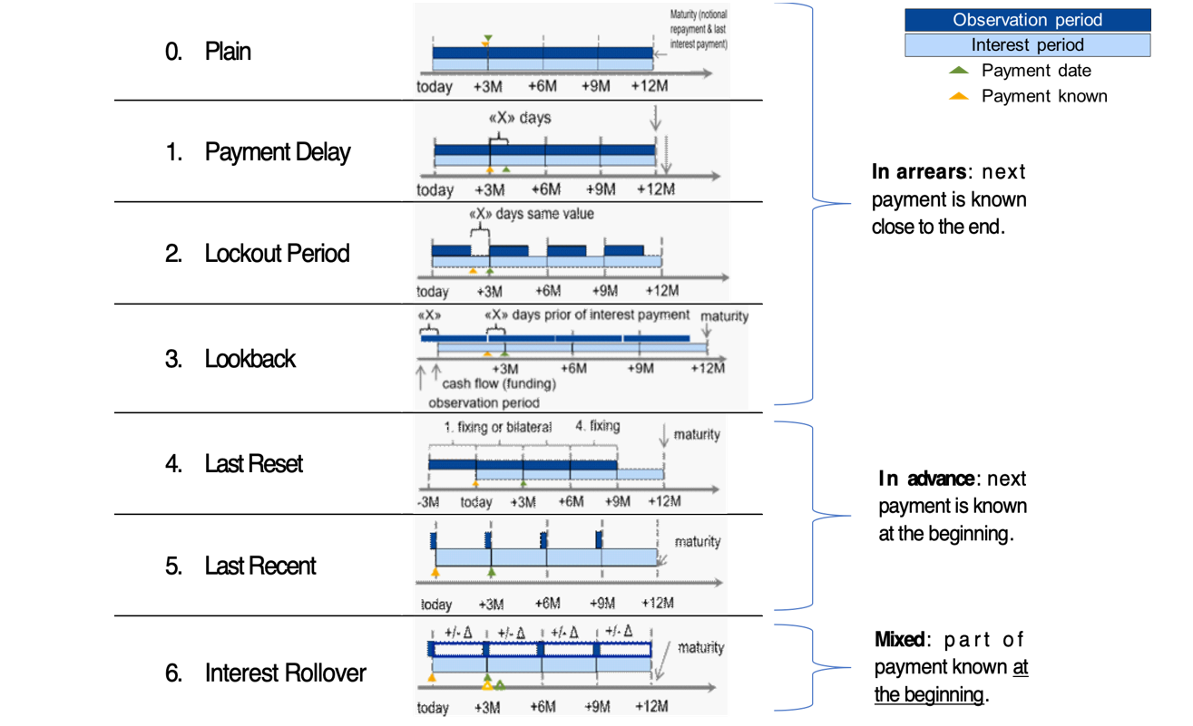
Figure 1: Overview of alternative techniques for calculating compounded SARON. Source: Financial Stability Board (2019).
0) Plain (in arrears): The observation period is identical to the interest period. The notional is paid at the start of the period and repaid on the last day of the contract period together with the last interest payment. Moreover, a Plain (in arrears) structure reflects the movement in interest rates over the full interest period and the payment is made on the day that it would naturally be due. On the other hand, given publication timing for most RFRs (T+1), the requiring payment is on the same day (T+1) that the final payment amount is known (T+1). An exception is SARON, as SARON is published one business day (T+0) before the overnight loan is repaid (T+1).
Example: the 1-month compounded SARON based on the Plain technique is like the example explained in the previous article, but has a different start date (1 February 2019). The resulting 1-month compounded SARON is equal to -0.7340% and it is known one day before the payment date (i.e. known on 28 February 2019).
1) Payment Delay (in arrears): Interest rate payments are delayed by X days after the end of an interest period. The idea is to provide more time for operational cash flow management. If X is set to 2 days, the cash flow of the loan matches the cash flow of most OIS swaps. This allows perfect hedging of the loan. On the other hand, the payment in the last period is due after the payback of the notional, which leads to a mismatch of cash flows and a potential increase in credit risk.
Example: the 1-month compounded SARON is equal to -0.7340% and like the one calculated using the Plain (in arrears) technique. The only difference is that the payment date shifts by X days, from 1 March 2019 to e.g. 4 March 2019. In this case X is equal to 3 days.
2) Lockout Period (in arrears): The RFR is no longer updated, i.e. frozen, for X days prior to the end of an interest rate period (lockout period). During this period, the RFR on the day prior to the start of the lockout is applied for the remaining days of the interest period. This technique is used for SOFR-based Floating Rate Notes (FRNs), where a lockout period of 2-5 days is mostly used in SOFR FRNs. Nevertheless, the calculation of the interest rate might be considered less transparent for clients and more complex for product providers to be implemented. It also results in interest rate risk that is difficult to hedge due to potential changes in the RFR during the lockout period. The longer the lockout period, the more difficult interest rate risk can be hedged during the lockout period.
Example: the 1-month compounded SARON with a lockout period equal to 3 days (i.e. X equals 3 days) is equal to -0.7337% and known 3 days in advance of the payment date.
3) Lookback (in arrears): The observation period for the interest rate calculation starts and ends X days prior to the interest period. Therefore, the interest payments can be calculated prior to the end of the interest period. This technique is predominately used for SONIA-based FRNs with a delay period of X equal to 5 days. An increase in interest rate risk due to changes in yield curve is observed over the lifetime of the product. This is expected to make it more difficult to hedge interest rate risk.
Example: assuming X is equal to 3 days, the 1-month compounded SARON would start in advance, on January 29, 2019 (i.e. today minus 3 days). This technique results in a compounded 1-month SARON equal to -0.7335%, known on 25 February 2019 and payable on 1 March 2019.
4) Last Reset (in advance): Interest payments are based on compounded RFR of the previous period. It is possible to ensure that the present value is equivalent to the Plain (in arrears) case, thanks to a constant mark-up added to the compounded RFR. The mark-up compensates the effects of the period shift over the full life of the product and can be priced by the OIS curve. In case of a decreasing yield curve, the mark-up would be negative. With this technique, the product is more complex, but the interest payments are known at the start of the interest period, as a LIBOR-based product. For this reason, the mark-up can be perceived as the price that a borrower is willing to pay due to the preference to know the next payment in advance.
Example: the interest rate payment on 1 March 2019 is already known at the start date and equal to -0.7328% (without mark-up).
5) Last Recent (in advance): A single RFR or a compounded RFR for a short number of days (e.g. 5 days) is applied for the entire interest period. Given the short observation period, the interest payment is already known in advance at the start of each interest period and due on the last day of that period. As a consequence, the volatility of a single RFR is higher than a compounded RFR. Therefore, interest rate risk cannot be properly hedged with currently existing derivatives instruments.
Example: a 5-day average is used to calculate the compounded SARON in advance. On the start date, the compounded SARON is equal to -0.7339% (known in advance) that will be paid on 1 March 2020.
6) Interest Rollover (hybrid): This technique combines a first payment (installment payment) known at the beginning of the interest rate period with an adjustment payment known at the end of the period. Like Last Recent (in advance), a single RFR or a compounded RFR for a short number of days is fixed for the whole interest period (installment payment known at the beginning). At the end of the period, an adjustment payment is calculated from the differential between the installment payment and the compounded RFR realized during the interest period. This adjustment payment is paid (by either party) at the end of the interest period (or a few days later) or rolled over into the payment for the next interest period. In short, part of the interest payment is known already at the start of the period. Early termination of contracts becomes more complex and a compensation mechanism is needed.
Example: similar to Last Recent (in advance), a 5-day compounded SARON can be considered as installment payment before the starting date. On the starting date, the 5-day compounded SARON rate is equal to -0.7339% and is known to be paid on 1 March 2019 (payment date). On the payment date, an adjustment payment is calculated as the delta between the realized 1-month compounded SARON, equal to -0.7340% based on Plain (in arrears), and -0.7339%.
There is a trade-off between knowing the cash flows in advance and the desire for a payment structure that is fully hedgeable against realized interest rate risk. Instruments in the derivatives market currently use ‘in arrears’ payment structures. As a result, the more the option used for a cash product deviates from ‘in arrears’, the less efficient the hedge for such a cash product will be. In order to use one or more of these options for cash products, operational cash management (infrastructure) systems need to be updated. For more details about the calculation of the compounded SARON using the alternative techniques, please refer to Table 1 and Table 2 in the Appendix I. The compounding formula used in the calculation is explained in the previous article.
Overall, market participants are recommended to consider and assess all the options above. Moreover, the financial institutions should individually define action plans with respect to their own product strategies.
Conclusions
The transition from IBOR to alternative reference rates affects all financial institutions from a wide operational perspective, including how products are created. Existing LIBOR-based cash products need to be replaced with SARON-based products as the mortgages contract. In the next installment, IBOR Reform in Switzerland – Part III, the latest information from the Swiss National Working Group (NWG) and market developments on the compounded SARON will be explained in more detail.
Contact
For more information about the challenges and latest developments on SARON, please contact Martijn Wycisk or Davide Mastromarco of Zanders’ Swiss office: +41 44 577 70 10.
The other articles on this subject:
Transition from CHF LIBOR to SARON, IBOR Reform in Switzerland, Part I
Compounded SARON and Swiss Market Development, IBOR Reform in Switzerland, Part III
Fallback provisions as safety net, IBOR Reform in Switzerland, Part IV
References
- Mastromarco, D. Transition from CHF LIBOR to SARON, IBOR Reform in Switzerland – Part I. February 2020.
- National Working Group on Swiss Franc Reference Rates. Discussion paper on SARON Floating Rate Notes. July 2019.
- National Working Group on Swiss Franc Reference Rates. Executive summary of the 12 November 2019 meeting of the National Working Group on Swiss Franc Reference Rates. Press release November 2019.
- National Working Group on Swiss Franc Reference Rates. Starter pack: LIBOR transition in Switzerland. December 2019.
- Financial Stability Board (FSB). Overnight Risk-Free Rates: A User’s Guide. June 2019.
- ISDA. Supplement number 60 to the 2006 ISDA Definitions. October 2019.
- ISDA. Interbank Offered Rate (IBOR) Fallbacks for 2006 ISDA Definitions. December 2019.
- National Working Group on Swiss Franc Reference Rates. Executive summary of the 7 May 2020 meeting of the National Working Group on Swiss Franc Reference Rates. Press release May 2020

With the advance of the current low interest rate environment and increased regulatory requirements, modeling mortgages for valuation purposes is more complex. Additionally, the applicable valuation method depends on the purpose of the valuation.
The most common valuation method for mortgage funds is known as the ‘fair value’ method, consisting of two building blocks: the cash flows and a discount curve. The first prerequisite to apply the fair value method is to determine future cash flows, based on the contractual components and behavioral modeling. The other prerequisite is to derive the appropriate rate for discounting via a top-down or bottom-up approach.
Two building blocks
The appropriate approach and level of complexity in the mortgage valuation depend on the underlying purpose. Examples of valuation purposes are: regulatory, accounting, risk or sales of the mortgage portfolio. For example BCBS, IRRBB, Solvency, IFRS and the EBA ask for (specific) valuation methods of mortgages. The two building blocks for a ‘fair value’ calculation of mortgages are expected cash flows and a discount curve.
The market value is the sum of the expected cash flows at the moment of valuation, which are derived by discounting future expected cash flows with an appropriate curve. For both building block models, choices have to be made resulting in a tradeoff between the accuracy level and the computational effort.
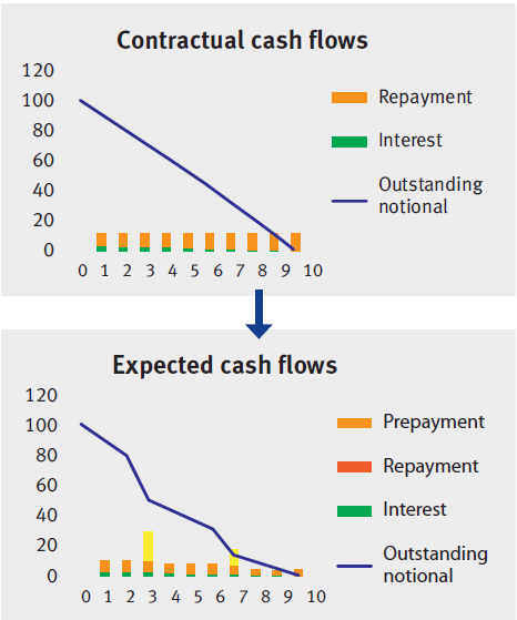
Figure 1: Constructing the expected cash flows from the contractual cash flows for a loan with an annuity repayment type.
Cash flow schedule
The contractual cash flows are projected cash flows, including repayments. These can be derived based on the contractually agreed loan components, such as the interest rate, the contractual maturity and the redemption type.
The three most commonly used redemption types in the mortgage market are:
- Bullet: interest only payments, no contractual repayment cash flows except at maturity
- Linear: interest (decreasing monthly) and constant contractual repayment cash flows
- Annuity: fixed cash flows, consisting of an interest and contractual repayment part
However, the expected cash flows will most likely differ from this contractually agreed pattern due to additional prepayments. Especially in the current low interest rate environment, borrowers frequently make prepayments on top of the scheduled repayments.
Figure 1 shows how to calculate an expected cash flow schedule by adding the prepayment cash flows to the contractual cash flow. There are two methods to derive : client behavior dependent on interest rates and client behavior independent of interest rates. The independent method uses an historical analysis, indicating a backward looking element. This historical analysis can include a dependency on certain contract characteristics.
On the other hand, the interest rate dependent behavior is forward looking and depends on the expected level of the interest rates. Monte Carlow simulations can model interest dependent behavior.
Another important factor in client behavior are penalties paid in case of a prepayment above a contractually agreed threshold. These costs are country and product specific. In Italy, for example, these extra costs do not exist, which could currently result in high prepayments rates.
Discount curve
The curve used for cash flow discounting is always a zero curve. The zero curve is constructed from observed interest rates which are mapped on zero-coupon bonds to maturities across time. There are three approaches to derive the rates of this discount curve: the top down-approach, the bottom-up approach or the negotiation approach. The first two methods are the most relevant and common.
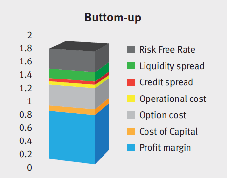
In theory, an all-in discount curve consists of a riskfree rate and several spread components. The ‘base’ interest curve concerns the risk-free interest rate term structure in the market at the valuation date with the applicable currency and interest fixing frequency (or use ccy- and basis-spreads). The spreads included depend on the purpose of the valuation. For a fair value calculation, the following spreads are added: liquidity spread, credit spread, operational cost, option cost, cost of capital and profit margin. An example of spreads included for other valuation purposes are offerings costs and origination fee.
Top-down versus Bottom-up
The chosen calculation approach depends on the available data, the ability to determine spread components, preferences and the purpose of the valuation.
A top-down method derives the applied rates of the discount curve from all-in mortgage rates on a portfolio level. Different rates should be used to construct a discount curve per mortgage type and LTV level, and should take into account the national guaranteed amount (NHG in the Netherlands). Subtract all-in mortgage rates spreads that should not part of the discount curve, such as the offering costs. Use this top-down approach when limited knowledge or tools are available to derive all the individual spread components. The all-in rates can be obtained from the following sources: mortgage rates in the market, own mortgage rates or by designing a mortgage pricing model.
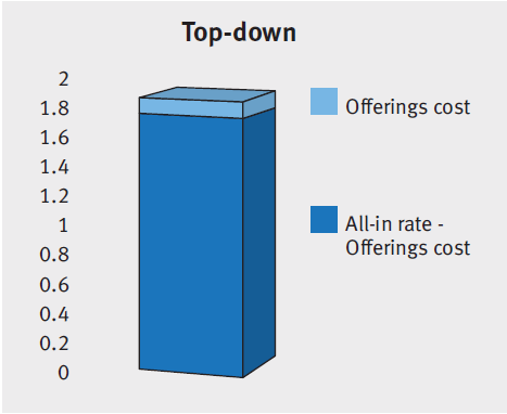
Figure 2
The bottom-up approach constructs the applied discount curve by adding all applicable spreads on top of the zero curve at a contract level. This method requires that several spread components can be calculated separately. The top-down approach is quicker, but less precise than the bottom-up approach, which is more accurate but also computationally heavy. Additionally, the bottom-up method is only possible if the appropriate spreads are known or can be derived. One example of a derivation of a spread component is credit spreads determined from expected losses based on an historical analysis and current market conditions.
In short
A fair value calculation performed by a discounted cash flow method consists of two building blocks: the expected cash flows and a discount curve. This requires several model choices before calculating a fair value of a mortgage (portfolio).
The expected cash flow model is based on the contractual cash flows and any additional prepayments. The mortgage prepayments can be modeled by assuming interest dependent or interest independent client behavior.
To construct the discount curve, the relevant spreads should be added to the risk-free curve. The decision for a top-down or bottom-up approach depends on the available data, the ability to determine spread components, preferences and the purpose of the valuation.
These important choices do not only apply for fair value calculations but are applicable for many other mortgage valuation purposes.
Zanders Valuation Desk
Independent, high quality, market practice and accounting standard proof are the main drivers of our Valuation Desk. For example, we ensure a high quality and professionalism with a strict, complete and automated check on the market data from our market data provider on a daily basis. Furthermore, we have increased our independence by implementing the F3 solution from FINCAD in our current valuation models. This permits us to value a larger range of financial instruments with a high level of quality, accuracy and wider complexity.
For more information or questions concerning valuation issues, please contact Pierre Wernert: [email protected].


Although the general accounting mechanisms will largely remain unchanged, the long waited reforms of IFRS 9 encompass an array of changes that will influence your hedge accounting process in different ways.
Cross-currency interest rate swaps (CC-IRS), options, FX forwards and commodity trades are just a few examples of financial instruments which will be affected by the upcoming changes. The time value, forward points and cross-currency basis spread will receive different accounting treatment under IFRS 9. Within Zanders, we feel the need to clarify these key changes that deserve as much awareness as possible.
1. Accounting for the forward element in foreign currency forwards
Each FX forward contract possesses a spot and forward element. The forward element represents the interest rate differential between the two currencies. Under IFRS 9 (similar to IAS 39), it is allowed to designate the entire contract or just the spot component as the hedging instrument. When designating the spot component only, the change in fair value of the forward element is recognised in OCI and accumulated in a separate component of equity. Simultaneously, the fair value of the forward points at initial recognition is amortised, most expected linearly, over the life of the hedge.
Again, this accounting treatment is only allowed in case the critical terms are aligned (similar). If at inception the actual value of the forward element exceeds the aligned value, changes in the fair value based on the aligned item will go through OCI. The difference between the fair value of the actual and aligned forward elements is recognized in P&L. In case the value of the aligned forward element exceeds the actual value at inception, changes in fair value are based on the lower of aligned versus actual and go to OCI. The remaining change of actual will be recognized in P&L.
Please refer to the example below:
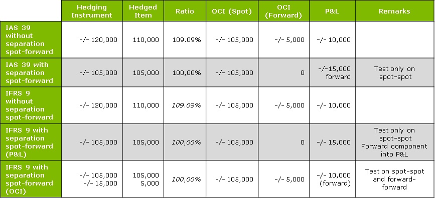
In this example, we consider an entity X which is hedging a future receivable with an FX forward contract.
MtM change of the forward = 105,000 (spot element) + 15,000 (forward element) = 120,000.
MtM change of the hedged item = 105,000 (spot element) + 5,000 (forward element) = 110,000.
We look at alternatives under IAS39 and IFRS9 that show different accounting methods depending on the separation between the spot and forward rates.
Under IAS39 and without a spot/forward separation, the hedging instrument represents the sum of the spot and the forward element (105 000 spot + 15 000 forward= 120 000). The hedged item consisting of 105 000 spot element and 5 000 forward element and the hedge ratio being within the boundaries, the minimum between the hedging instrument and hedged item is listed as OCI, and the difference between the hedging instrument and the hedged item goes to the P&L.
However, with the spot/forward separation under IAS39, the forward component is not included in the hedging relationship and is therefore taken straight to the P&L. Everything that exceeds the movement of the hedged item is considered as an “over hedge” and will be booked in P&L.
Line 3 and 4 under IFRS9 characterise comparable registration practices than under IAS39. The changes come in when we examine line 5, where the forward element of 5 000 can be registered as OCI. In this case, a test on both the spot and the forward element is performed, compared to the previous line where only one test takes place.
2. Rebalancing in a commodity hedge relation
Under influence of changing economic circumstances, it could be necessary to change the hedge ratio, i.e. the ratio between the amount of hedged item and the amount of hedging instruments. Under IAS 39, changes to a hedge ratio require the entity to discontinue hedge accounting and restart with a new hedging relationship that captures the desired changes. The IFRS 9 hedge accounting model allows you to refine your hedge ratio without having to discontinue the hedge relationship. This can be achieved by rebalancing.
Rebalancing is possible if there is a situation where the change in the relationship of the hedging instrument and the hedged item can be compensated by adjusting the hedge ratio. The hedge ratio can be adjusted by increasing or decreasing either the number of designated hedging instruments or hedged items.
When rebalancing a hedging relationship, an entity must update its documentation of the analysis of the sources of hedge ineffectiveness that are expected to affect the hedging relationship during its remaining term.
Please refer to the example below:
Entity X is hedging a forecast receivable with a FX call.
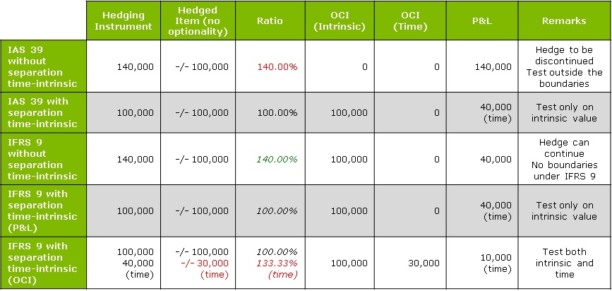
MtM change of the option = 100,000 (intrinsic value) + 40,000 (time value) = 140,000.
MtM change of the hedged item = 100,000 (intrinsic value) + 30,000 (time value) = 130,000.
In example 3, we consider entity X to be hedging a forecast receivable via an FX call. Note that under IAS39 the hedged item cannot contain an optionality if this optionality is not present in the underlying exposure. Hence, in this example, the hedged item cannot contain any time value. The time value of 30,000 can be used under IFRS9, but only by means of a separate test (see row 5).
In line 1, we can see that without a time-intrinsic separation, the hedge relationship is no longer within the 80-125% boundary; therefore, it needs to be discontinued and the full MtM has to be booked in the P&L. In line 2, there is a time-intrinsic separation, and the 40 000 representing the time value of the option are not included in the hedge relationship, meaning that they go straight to the P&L.
Under IFRS9 with no time-intrinsic separation (line 3), the hedging relationship is accounted for in the usual manner, as the ineffectiveness boundary is not applicable, with 100 000 going representing OCI, and the over hedged 40 000 going to the P&L.
However, the time-intrinsic separation under IFRS9 in line 4 is similar to line 2 under IAS39, in which we choose to immediately remove the time value for the option from the hedging relationship. We therefore have to account for 40 000 of time value in the P&L.
In the last line, we separate between time and intrinsic values, but the time value of the option is aimed to be booked into OCI. In this case, a test on both the intrinsic and the time element is performed. We can therefore comprise 100 000 in the intrinsic OCI, 30 000 in the time OCI, and 10 000 as an over hedge in the P&L.
4. Cross-currency basis spread are considered a cost of hedging
The cross-currency basis spread can be defined as the liquidity premium of one currency over the other. This premium applies to exchanges of currencies in the future, e.g. a hedging instrument like an FX forward contract. If a cross currency interest rate swap is used in combination with a single currency hedged item, for which this spread is not relevant, hedge ineffectiveness could arise.
In order to cope with this mismatch, it has been decided to expand the requirements regarding the costs of hedging. Hedging costs can be seen as cost incurred to protect against unfavourable changes. Similar to the accounting for the forward element of the forward rate, an entity can exclude the cross-currency basis spread and account for it separately when designating a hedging instrument. In case a hypothetical derivative is used, the same principle applies. IFRS 9 states that the hypothetical derivative cannot include features that do not exist in the hedged item. Consequently, cross-currency basis spread cannot be part of the hypothetical derivative in the previously mentioned case. This means that hedge ineffectiveness will exist.
Please refer to the example below:
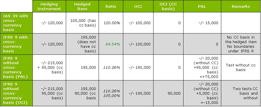
In example 4, we consider an entity X hedging a USD loan with a CCIRS.
MtM change of CCIRS = 215,000 – 95,000 (cross-currency basis) = 120,000.
MtM change hedged = 195,000 – 90,000 (cross-currency basis) = 105,000.
Under IAS39, there is only one way to account for CCIRS. The full amount of 120 000 (including the – 95 000 cross-currency basis) is considered as the hedging instrument, meaning that 105 000 can be listed as OCI and 15 000 of over hedge have to go to the P&L.
Under IFRS9, there is the option to exclude the cross-currency basis and account for it separately.
In line 2, we can see the conditions under IFRS9 when a cross-currency basis is included: the cross-currency basis cannot be comprised in the hedged item, so there is an under hedge of 75 000.
In line 3, we exclude the cross-currency basis from the test for the hedging instrument. By registering the MtM movement of 195 000 as OCI, we then account for the 95 000 of cross-currency basis, as well as -/- 20 000 of over hedge in the P&L. In line 4, the cross-currency basis is included in a separate hedge relationship – we therefore perform an extra test on the cross-currency basis (aligned versus actual values) . From the first test, -/- 195,000 is registered as OCI and -/- 20,000 (“over hedge” part) in P&L; from the cross-currency basis test 90,000 represents OCI and 5,000 has to be included in P&L.

Ballast Nedam, with support from Zanders’ expertise in hedge accounting and financial valuation, effectively manages financial risks in long-term infrastructure projects through public-private partnerships.
Building houses, mobility, energy and nature – these are the areas in which Ballast Nedam is active. Customers are large and middle-sized companies, private and public. In addition to building roads and houses, the company installs foundations for offshore wind farms, invests in alternative fuel, extracts gravel, and works to make homes more sustainable. Ballast Nedam aims to be involved in the entire life cycle of projects – development, realization, management, recycling, and funding. This enables an integral approach.
An example is the approach of highway A2 through Maastricht, commissioned by the Ministry of Infrastructure and the Environment, where Ballast Nedam, as part of the combination Avenue 2, is working on an integral solution. The tunnel roof of the dual-layered tunnel will become at a later stage a green strip of nature that reconnects the different city parts of Maastricht. Large projects like these will in most cases be executed through a consortium with other contractors, to spread the risk. Just like the Kromhout military base in Utrecht, a project for the Ministry of Defense, with a value of more than EUR 450 million on an area of 19 hectares.
Life cycle thinking and doing
A public-private partnership (PPP), such as the Kromhout military base, is a form of cooperation between the government and one or more parties. In an increasing number of cases, Ballast Nedam is also taking on the responsibility, after the building phase, of management and maintenance. Such outsourcing of the management means clarity and cost savings for the government. For the construction firm, it is a secure source of income, which in certain cases also increases the room to maneuver when designing the project.
In another PPP-project for the construction of the A15 Maasvlakte-Vaanplein highway, the government posed a mobility question and requested a complete solution, starting with a list of concrete demands. This project is about the widening of the A15 at a busy section and the building of a new Botlek bridge. Ballast Nedam is part of the consortium A-Lanes A15, which is responsible for the design, building, and funding of the project plus 20 years of maintenance, with a value of approximately EUR 1.5 billion. Because of the management component, such projects last longer, sometimes even 30 years.
“These sorts of requests, where the government engages in a contract for many years and outsources the management, are relatively new,” explains Bart Buyck, financial controller at Ballast Nedam Concessions.
They have been in the market for about 10 years and have seen strong growth in this sort of contract in the past five years. That is why Ballast Nedam established its Concessions arm to focus on what we call ‘life cycle projects,’ public-private partnerships with a long completion time. Concessions acts within Ballast Nedam as financier. So how can Ballast Nedam finance these large long-duration projects?
Thinking outside the box
For every PPP-project, a Special Purpose Company (SPC) is established. The project is based around that SPC, which is the link between customer, financier, shareholder (Ballast Nedam and other investors), builder, and manager. With all these parties, the SPC concludes agreements. A PPP-project, with a contract value of sometimes hundreds of millions of euros, will for the largest part – 80-90 percent – be funded privately, by a bank. Depending on the size and the risk of the project, Ballast Nedam is involved in a certain portion, varying from 20 to 100 percent.
Ballast Nedam Concessions acts in the SPC as project manager, quality assurance manager, and process manager. Preferably, it will assume responsibility for the entire project. “In that case, you can make a difference at bids,” Buyck says. “If you continue to think inside the box, you will not achieve optimization. Designer, builder, and manager should decide together what the smartest, most efficient solution is. Only by doing so will you be able to break out of the box.”
Interest rate swaps
For the duration of the contract, the customer periodically pays a fixed amount of interest, repayment, and services. Buyck says: “An interest component is included on the customer’s invoice. When offering a PPP-project, you need to consider the impact of that interest rate and hence fix it. The funding is based on a floating interest rate. Because you receive a fixed interest rate and pay a floating interest, an interest rate risk arises. This risk limits financing possibilities and can have a negative effect on the return. To hedge interest rate risks, the SPC concludes an interest rate swap: it pays a fixed rate to the bank and receives a floating interest rate in return. That is how one can hedge that sort of risk.”
With hedged risks, all parties involved know where they stand. But from an accounting perspective, not all conditions will have been met. Ballast Nedam reports as a listed company under IFRS (International Financial Reporting Standards). IFRS contains rules for the preparation of annual statements and for other periodical financial reporting.
That is the moment when the expertise of Zanders Valuation Desk is required.
Bart Buyck, financial controller at Ballast Nedam Concessions.
“At this moment we have five of this kind of SPCs. In 2008 we were confronted for the first time with IFRS requirements with regard to the valuation of interest rate hedges on SPCs. We engaged Zanders at that time to value the interest rate swaps. Together we set up and refined the methodology.”
Hedge Accounting
Derivatives like interest-rate swaps have to be valued in the books at market value in accordance with IAS 39. Changes in market value must be accounted for in the profit and loss account. This can cause undesired temporary volatility in the result. To remedy that, IAS 39 allows for hedge accounting; a company can – provided certain conditions are met – put the market value of derivatives temporarily on its balance sheet.
Buyck notes: “Every quarter Zanders performs two things for us. Firstly, they determine the market value of the instrument using current yield curves. Secondly, they apply hedge accounting; they use an effectiveness test to determine the degree to which the hedge instrument is still in line with the premises on which it was originally concluded and the underlying funding position. We provide them with our loan positions and the forecasts for the future.”
If you do not apply hedge accounting, you must account for changes in market value in your profit and loss account. If you do apply hedge accounting and you comply with the requirements, you may put it as a provision on your balance sheet. “It is a very technical and specific area,” Buyck says. “All sorts of things are involved in this; the valuation methodology, the accounting in connection with that and finally the financial reporting both internally and vis-à-vis the auditor. But it does create transparency. Thanks to swaps – while causing accounting complexity – we have secure cash flows. This will make it easier to find funding for all the great projects we are still going to do.”
Zanders’ Valuation Desk provides and validates valuations of financial products for all market segments. In addition, experts study the financial markets and analyze market developments. The valuations and analyses of the Valuation Desk are objective and independent. The services of the Valuation Desk include periodic valuations (for example for commodity derivatives), hedge accounting, research, and support when calculating margin calls.
Would you like to know more? Contact us today.

Derivatives are often used to mitigate or offset risks (such as interest or currency risk) that arise from corporate activities. The standard accounting treatment for hedge instruments is that changes in fair value will have to be recorded in Profit and Loss (P&L). As opposed to the hedge instruments, the hedged assets or liabilities are often measured at (amortized) cost or fair value through equity, or are forecasted items which are not recognized in the Balance Sheet.
This results in a (temporary) valuation and or timing; mismatch between the hedged item and the hedge instrument. The objective of hedge accounting is to avoid temporary undesired volatility in P&L as a result of these valuation and timing differences. However, entities can practice hedge accounting only if they meet the numerous and complex requirements set out in IAS 39. What are these requirements and how Zanders can help you in the different steps?
What is hedging?
The aim of hedging is to mitigate the impact of non-controllable risks on the performance of an entity. Common risks are foreign exchange risk, interest rate risk, equity price risk, commodity price risk and credit risk.
The hedge can be executed through financial transactions. Examples in which hedging is used include:
- an entity that has a liability in a foreign currency and wants to protect itself against the change in the foreign exchange rate
- a company entering into an interest rate swap so that the floating rate of a loan becomes a fixed rate
Types of hedge accounting
There are three types of hedge accounting: fair value hedges, cash flow hedges and hedges of the net investment in a foreign operation.
- Fair Value Hedge
The risk being hedged in a fair value hedge is a change in the fair value of an asset or a liability. For examples, changes in fair value may arise through changes in interest rates (for fixed-rate loans), foreign exchange rates, equity prices or commodity prices. - Cash Flows Hedges
The risk being hedged in a cash flow hedge is the exposure to variability in cash flows that is attributable to a particular risk and could affect the income statement. Volatility in future cash flows will result from changes in interest rates, exchange rates, equity prices or commodity prices. - Hedges of net investment in a foreign operation
An entity may have overseas subsidiaries, associates, joint ventures or branches (‘foreign operations’). It may hedge the currency risk associated with the translation of the net assets of these foreign operations into the group’s currency. IAS 39 permits hedge accounting for such a hedge of a net investment in a foreign operation.
The mismatch in the income statement recognition
Under the accounting standard IAS 39, all derivatives are recorded at fair value in the income statement. However these derivatives are often used to hedge recognized assets and liabilities, which are recorded at amortized cost or forecasted transactions that are not yet recognized on the Balance Sheet yet. The difference between the fair value measurement for the derivative and the amortized cost for the asset/liability leads to a mismatch in the timing of income statement recognition.
Hedge accounting seeks to correct this mismatch by changing the timing recognition in the income statement. Fair value hedge accounting treatment will accelerate the recognition of gains or losses on the hedged item into the P&L, whereas cash flow hedge accounting and net investment hedge accounting will defer the gains or losses on the hedge instrument.
The hedge relation
The hedge relation consists of a hedged item and a hedge instrument. A hedged item exposes the entity to the risk of changes in fair value or future cash flows that could affect the income statement currently or in the future. For example, a hedged item could be a loan in which the entity is paying a floating rate (e.g., Euribor 6 month + spread) to a counterparty.
If the hedge instrument is a derivative, it can be designated entirely or as a proportion as a hedging instrument. Even a portfolio of derivatives can be jointly designated as a hedge instrument. The hedge instrument can be a swap in which the entity is receiving a floating rate and paying a fixed rate. With this relation the entity is offsetting the floating rate payments and will only pay the fixed rate.
Criteria to qualify for hedge accounting
Hedge accounting is an exception to the usual accounting principles, thus it has to meet several criteria:
- At the start of the hedge, the hedged item and the hedging instrument has to be identified and designated.
- At the start of the hedge, the hedge relationship must be formally documented.
- At the start of the hedge, the hedge relationship must be highly effective.
- The effectiveness of the hedge relationship must be tested periodically. Ineffectiveness is allowed, provided that the hedge relationship achieves an effectiveness ratio between 80% and 125%.
Hedge effectiveness
Complying with IAS 39 requires two types of effectiveness tests:
- A prospective (forward-looking) test to see whether the hedging relationship is expected to be highly effective in future periods
- A retrospective (backward-looking) test to assess whether the hedging relationship has actually been highly effective in past periods
Both tests need to be highly effective at the start of the hedge. A prospective test is highly effective if, at the inception of the hedge relation and during the period for which the hedge relation is designated, the expected changes in fair value of cash flows are offset. Meaning that during the life of the hedge relation, the change in fair value (due to change in the market conditions) of the hedged item should be offset by the change in fair value of the hedged instrument.
A retrospective test is highly effective if the actual results of the hedge are within the range 80%-125%.
Calculation methods
IAS 39 does not specify a single method for the calculation of the effectiveness of the hedge. The method used depends on the risk management strategy. The most common methods are:
- Critical terms comparison – this method consists of comparing the critical terms (notional, term, timing, currency, and rate) of the hedging instrument with those from the hedged item. This method does not require any calculation.
- Dollar offset method – this is a quantitative method that consists of comparing the change in fair value between the hedging instrument and the hedged item. Depending on the entity risk policies, this method can be performed on a cumulative basis (from inception) or on a period-by-period basis (between two specific dates). A hedge is considered highly effective if the results are within the range 80%-125%.
- Regression analysis – this statistical method investigates the strength of the statistical relationship between the hedged item and the hedge instrument. From an accounting perspective this method proves whether or not the relationship is sufficiently effective to qualify for hedge accounting. It does not calculate the amount of ineffectiveness.
Termination of the hedge relation
A hedge relation has to be terminated going forward when any of the following occur:
- A hedge fails an effectiveness test
- The hedged item is sold or settled
- The hedging instruments are sold, terminated or exercised
- Management decides to terminate the relation
- For a hedge of a forecast transaction; the forecast transaction is no longer highly probable.
Please note that these requirements described previously may change as the IASB is currently working to replace IAS39 by IFRS9 (new qualification of hedging instruments, hedged items, hedge effectiveness…)
Conclusion
Hedge accounting is a complex process involving numerous and technical requirements with the objective to avoid temporary undesired volatility in P&L. This volatility is the result of valuation and or timing mismatch between the hedged item and the hedge instrument. If you are considering hedge accounting, we have a dedicated team on the valuation desk. We can offer advices on the calculation of the market values of the underlying risks and the hedge instruments, as well as setting up the hedge relation, preparing documentation and helping on the accounting treatment of the results.
You can implement hedge accounting with Kantox Edge Accounting Powered by Zanders. It's the latest in hedge accounting software paired with expert implementation support from Zanders.

Since the first transaction in 1981 between the World Bank and IBM, the market of cross-currency swaps has grown rapidly. It represents, according to the Bank of International Settlements, an outstanding notional amount of USD 16,347 billion as per June 2010. In this article we will discuss how cross-currency swaps work, and how to value them.
A cross-currency swap (CCS), can have different objectives. It can reduce the exposure to exchange rate fluctuation or it can provide arbitrage opportunities between different rates. It can be used for example, if a European company is looking to acquire some US dollar bonds but does not want to expose itself to US dollar risk. In this case it is possible to do a CCS transaction with a US-based bank. The European company is paying in euros and receives a (fixed) US dollar cash flow. With these flows the European company can meet its US dollar obligations.
The valuation of a CCS is quite similar to the valuation of an interest-rate swap. The CCS is valued by discounting the future cash flows for both legs at the market interest rate applicable at that time. The sum of the cash flows denoted in the foreign currency (hereafter euro) is converted with the spot rate applicable at that time. One big difference with an interest-rate swap is that a CCS always has an exchange of notional.
Looking at a CCS with a fixed-fixed structure (both legs of the swap have a fixed rate), the undiscounted cash flows are already known at the start of the deal, they are simply the product of the notional, the fixed rate and the year fraction.
The discounting of the cash flows requires a more complex method. The US dollar curve is the base of everything and is, therefore, not different from valuations of plain vanilla US dollar interest-rate swaps. Looking at a euro/US dollar CCS, the eurocurve (excluding credit spreads) is made of two parts:
- The euro interest rate curve and
- The basis spread.
This basis spread curve represents a ‘compensation’ for the changes in the forward FX rates between the two currencies used in the swap. Before the global credit crisis this spread was close to zero. Nowadays, the spread ranges from 18 basis points (bp) (10-year spread) to 40bp (one-year spread), but reached 120bp as shown by figure 1.
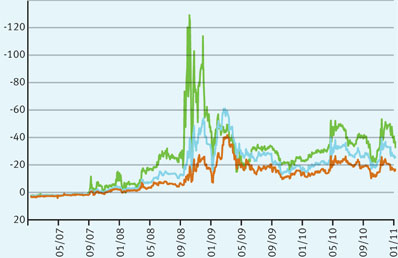
The big peak which is visible in the last quarter of 2008 was caused by the credit crisis (the default of Lehman Brothers and Bear Stearns, and the sale of Merrill Lynch, etc). Due to the lack of liquidity in the market during the crisis, the (liquidity) spreads in the US became a lot higher than those in Europe. To make up for this window of arbitrage, the basis spread decreased at a similar pace.
Here is an example: The characteristics of our USD-EUR example swap are:
The first leg in US dollar has a notional of USD 10,000,000 and a fixed interest of 2.50%
The valuation is performed at January 31st, 2011. The FX rate at that moment was EUR/USD 1.3697. The second leg in euro has a notional of EUR 7,481,670 and a fixed interest of 3.00%. The valuation is done from the perspective of the party which pays the euro flows and receives the US dollar flows. The frequency of the payment is annual and there is no amortization of the notional.
- In columns B and E the future cash flows are calculated by multiplying the notional with the fixed rate applicable for that leg. This results in cash flows of USD 250,000 (column B) and -/- EUR 224,450 (column E).
- The market value of the cash flows is calculated by multiplying the cash flows with their discount factor (column C for the US dollar and column F for the euro).
- The euro market value (column G) is converted to US dollar by multiplying it with the spot EUR/USD, i.e. 1.3697. Adding this converted value to the US dollar market value of column D results in the net market value (column H).
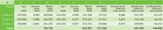
To demonstrate the impact of the basis spread we will repeat step 2 and 3 without the basis spread. The euro market value excluding basis spread is shown in column J, it is calculated by multiplying column E and I. The adjusted net market values are shown in column K. The difference of the sum of column H and K is 7,5 basis points of the US dollar notional. The basis spread impact can be checked, for the first year, by calculating the variation between the value in column G (222,206) with the value in column J (221,347), the result is 39bp which is in line with figure 1.
The above calculation shows that the exclusion of the basis spread in the valuation of the cross-currency swap results in a wrong net market value.
Get more of the resources you need in your inbox
You are currently viewing a placeholder content from HubSpot. To access the actual content, click the button below. Please note that doing so will share data with third-party providers.
More Information
Warren Buffet once called these products ‘weapons of mass destruction’, how do credit default swaps work?
Multi-billionaire Warren Buffet once called these products 'weapons of mass destruction', because he thought they were partly responsible for causing the credit crunch. Despite this remark, there is still a buoyant trade in credit default swaps. Here we discuss how they work, and how they are valued.
A credit default swap, or CDS, is effectively an insurance product whereby the consequences of a bankruptcy (default) of a reference party are transferred in return for a periodic payment. Take, for example, a party that wishes to purchase or has already purchased a bond, but is keen to avoid the (further) risk that the seller will go bankrupt. By concluding a CDS, any loss sustained in the case of default is compensated, or paid off, in return for a periodic payment; the premium for the CDS.
The CDS is valued in much the same way as its cousin, the interest rate swap. In an interest rate swap, the exchange of fixed and variable interest cash flows is valued by estimating the amount of the future cash flows in advance. These cash flows are then discounted at the market interest rate applicable at that time and added up. In the case of a CDS, two types of cash flow are also exchanged. Firstly, a series of cash flows from the risk seller to the risk buyer, including the periodic payment of the premium. These cash flows are then exchanged for a (possible) cash flow from risk buyer to risk seller in the event of a default. The periodic payment ceases immediately if that bankruptcy actually takes place.
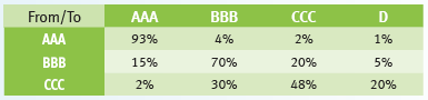
rating transition matrix
The greatest uncertainty in valuing a CDS is the moment of bankruptcy. This is generally determined by means of probability distribution and modeled on the basis of the ‘probability of default’ (PD). This probability can be obtained in the market by combining the rating of the bond with the rating transition matrix. These ratings are prepared by rating agencies. A triple-A rating is considered to denote ‘virtually risk-free’, a D rating means that a default event has already occurred. The matrix then indicates how great the probability is that a reference party will migrate from one rating to another.
Table 1 is a fictitious example of a rating transition matrix:
In order to illustrate the valuation of the CDS, we give an example of a credit default swap with the following assumptions:
- the term is two years,
- in case of bankruptcy, the loss is equal to the entire principal,
- the reference party’s current rating is BBB,
- we take the (fictitious) rating transition matrix from table 1, and
- the premium on the CDS is 4% of the principal.
Table 2 shows the probability distribution when calculating the moment of default:
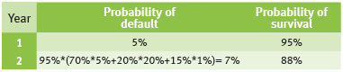
Explanation of table 2:
In year 1, the probability of default (the probability of migration from rating BBB to D) is: 5%. Taking into account this probability of default in that first year, the robability of bankruptcy in year 2 is 95%, multiplied by the following two-stage default probabilities:
- constant year 1 (BBB), followed by bankruptcy (70% x 5%),
- downgrade to CCC, followed by bankruptcy (20% x 20%), and
- upgrade to AAA, followed by bankruptcy (15% x1%).
The anticipated cash flows that are payable are equal to the premium in the first year (4) and 95% of the premium in the second year (95% x 4=3.8). The anticipated cash flows that are receivable are equal to 5% of the principal (5) in the first year and 7% of the principal in the second year (7).
Assuming an interest rate of 2% per year, the following calculations apply:
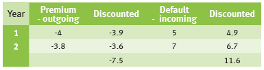
The market value of the CDS is positive because the discounted present value of the premium payments is lower than the anticipated payments in the case of bankruptcy.


