Recently, we have embarked on a process to align more effectively what we do with the changing needs of our clients in unprecedented times. A central pillar of this exercise was an in-depth dialogue with our clients and business partners around the world. These conversations confirmed that Zanders is trusted to translate our deep financial consultancy knowledge into solutions that answer the biggest and most complex problems faced by the world's most dynamic organizations. Our goal is to help these organizations withstand the current macroeconomic challenges and help them emerge stronger. Our purpose is grounded on the above.

"Zanders is trusted to translate our deep financial consultancy knowledge into solutions, answering the biggest and most complex problems faced by the world's most dynamic organizations."

Laurens Tijdhof

Our purpose is a reflection of what we do now, but it's also about what we need to do in the future.

It reflects our ongoing ambition - it's a statement of intent - that we should and will do more to affect positive change for both the shareholders of today and the stakeholders of tomorrow. We don't see that kind of ambition as ambitious; we see it as necessary.

The Zanders’ purpose is about the future. But it's also about where we find ourselves right now - a pandemic, high inflation and rising interest rates. And of course, climate change. At this year's Davos meeting, the latest Disruption Index was released showing how macroeconomic volatility has increased 200% since 2017, compared to just 4% between 2011 and 2016.

So, you have geopolitical volatility and financial uncertainty fused with a shifting landscape of regulation, digitalization, and sustainability. All of this is happening at once, and all of it is happening at speed.

The current macro environment has resulted in cost pressures and the need to discover new sources of value and growth. This requires an agile and adaptive approach. At Zanders, we combine a wealth of expertise with cutting-edge models and technologies to help our clients uncover hidden risks and capitalize on unseen opportunities.

However, it can't be solely about driving performance during stable times. This has limited value these days. It must be about delivering performance despite macroeconomic headwinds.

For over 30 years, through the bears, the bulls, and black swans, organizations have trusted Zanders to deliver financial performance when it matters most. We've earned the trust of CFOs, CROs, corporate treasurers and risk managers by delivering results that matter, whether it's capital structures, profitability, reputation or the environment. Our promise of "performance when it counts" isn't just a catchphrase, but a way to help clients drive their organizations, economies, and the world forward.

"For over 30 years, through the bears, the bulls, and black swans, financial guardians have trusted Zanders to deliver financial performance when it matters most."

Laurens Tijdhof

What "performance when it counts" means.

Navigating the current changing financial environment is easier when you've been through past storms. At Zanders, our global team has experts who have seen multiple economic cycles. For instance, the current inflationary environment echoes the Great Inflation of the 1970s. The last 12 months may also go down in history as another "perfect storm," much like the global financial crisis of 2008. Our organization's ability to help business and government leaders prepare for what's next comes from a deep understanding of past economic events. This is a key aspect of delivering performance when it counts.

The other side of that coin is understanding what's coming over the horizon. Performance when it counts means saying to clients, "Have you considered these topics?" or "Are you prepared to limit the downside or optimize the upside when it comes to the changing payments landscape, AI, Blockchain, or ESG?" Waiting for things to happen is not advisable since they happen to you, rather than to your advantage. Performance when it counts drives us to provide answers when clients need them, even if they didn't know they needed them. This is what our relationships are about. Our expertise may lie in treasury and risk, but our role is that of a financial performance partner to our clients.

How technology factors into delivering performance when it counts.

Technology plays a critical role in both Treasury and Risk. Real-time Treasury used to be an objective, but it's now an imperative. Global businesses operate around the clock, and even those in a single market have customers who demand a 24/7/365 experience. We help transform our clients to create digitized, data-driven treasury functions that power strategy and value in this real-time global economy.

On the risk management front, technology has a two-fold power to drive performance. We use risk models to mitigate risk effectively, but we also innovate with new applications and technologies. This allows us to repurpose risk models to identify new opportunities within a bank's book of business.

We can also leverage intelligent automation to perform processes at a fraction of the cost, speed, and with zero errors. In today's digital world, this combination of next generation thinking, and technology is a key driver of our ability to deliver performance in new and exciting ways.

"It’s a digital world. This combination of next generation of thinking and next generation of technologies is absolutely a key driver of our ability to deliver performance when it counts in new and exciting ways."

Laurens Tijdhof

How our purpose shapes Zanders as a business.

In closing, our purpose is what drives each of us day in and day out, and it's critical because there has never been more at stake. The volume of data, velocity of change, and market volatility are disrupting business models. Our role is to help clients translate unprecedented change into sustainable value, and our purpose acts as our North Star in this journey.

Moreover, our purpose will shape the future of our business by attracting the best talent from around the world and motivating them to bring their best to work for our clients every day.

"Our role is to help our clients translate unprecedented change into sustainable value, and our purpose acts as our North Star in this journey."

Laurens Tijdhof

ML models

ML models study a dataset and use the knowledge gained to make predictions for other datapoints. An ML model consists of an ML algorithm and one or more hyperparameters. ML algorithms study a dataset to make predictions, where hyperparameters determine the settings of the ML algorithm. The studying of a dataset is known as the training of the ML algorithm. Most ML algorithms have hyperparameters that need to be set by the user prior to the training. The trained algorithm, together with the calibrated set of hyperparameters, form the ML model.

ML models have different forms and shapes, and even more purposes. For selecting an appropriate ML model, a deeper understanding of the various types of ML that are available and how they work is required. Three types of ML can be distinguished:

• Supervised learning.
• Unsupervised learning.
• Semi-supervised learning.

The main difference between these types is the data that is required and the purpose of the model. The data that is fed into an ML model is split into two categories: the features (independent variables) and the labels/targets (dependent variables, for example, to predict a person’s height – label/target – it could be useful to look at the features: age, sex, and weight). Some types of machine learning models need both as an input, while others only require features. Each of the three types of machine learning is shortly introduced below.

Supervised learning

Supervised learning is the training of an ML algorithm on a dataset where both the features and the labels are available. The ML algorithm uses the features and the labels as an input to map the connection between features and labels. When the model is trained, labels can be generated by the model by only providing the features. A mapping function is used to provide the label belonging to the features. The performance of the model is assessed by comparing the label that the model provides with the actual label.

Unsupervised learning

In unsupervised learning there is no dependent variable (or label) in the dataset. Unsupervised ML algorithms search for patterns within a dataset. The algorithm links certain observations to others by looking at similar features. This makes an unsupervised learning algorithm suitable for, among other tasks, clustering (i.e. the task of dividing a dataset into subsets). This is done in such a manner that an observation within a group is more like other observations within the subset than an observation that is not in the same group. A disadvantage of unsupervised learning is that the model is (often) a black box.

Semi-supervised learning

Semi-supervised learning uses a combination of labeled and unlabeled data. It is common that the dataset used for semi-supervised learning consist of mostly unlabeled data. Manually labeling all the data within a dataset can be very time consuming and semi-supervised learning offers a solution for this problem. With semi-supervised learning a small, labeled subset is used to make a better prediction for the complete data set.

The training of a semi-supervised learning algorithm consists of two steps. To label the unlabeled observations from the original dataset, the complete set is first clustered using unsupervised learning. The clusters that are formed are then labeled by the algorithm, based on their originally labeled parts. The resulting fully labeled data set is used to train a supervised ML algorithm. The downside of semi-supervised learning is that it is not certain the labels are 100% correct.

Setting up the model

In most ML implementations, the data gathering, integration and pre-processing usually takes more time than the actual training of the algorithm. It is an iterative process of training a model, evaluating the results, modifying hyperparameters and repeating, rather than just a single process of data preparation and training. After the training is performed and the hyperparameters have been calibrated, the ML model is ready to make predictions.

Machine learning in financial risk management

ML can add value to financial risk management applications, but the type of model should suit the problem and the available data. For some applications, like challenger models, it is not required to completely explain the model you are using. This makes, for example, an unsupervised black box model suitable as a challenger model. In other cases, explainability of model results is a critical condition while choosing an ML model. Here, it might not be suitable to use a black box model.

In the next section we present some examples where ML models can be of added value in financial risk management.

Data quality analysis

All modeling challenges start with data. In line with the ‘garbage in, garbage out’ maxim, if the quality of a dataset is insufficient then an ML model will also not perform well. It is quite common that during the development of an ML model, a lot of time is spent on improving the data quality. As ML algorithms learn directly from the data, the performance of the resulting model will increase if the data quality increases. ML can be used to improve data quality before this data is used for modeling. For example, the data quality can be improved by removing/replacing outliers and replacing missing values with likely alternatives.

An example of insufficient data quality is the presence of large or numerous outliers. An outlier is an observation that significantly deviates from the other observations in the data, which might indicate it is incorrect. Outlier detection can easily be performed by a data scientist for univariate outliers, but multivariate outliers are a lot harder to identify. When outliers have been detected, or if there are missing values in a dataset, it might be useful to substitute some of these outliers or impute for missing values. Popular imputation methods are the mean, median or most frequent methods. Another option is to look for more suitable values; and ML techniques could help to improve the data quality here.

Multiple ML models can be combined to improve data quality. First, an ML model can be used to detect outliers, then another model can be used to impute missing data or substitute outliers by a more likely value. The outlier detection can either be done using clustering algorithms or by specialized outlier detection techniques.

Loan approval

A bank’s core business is lending money to consumers and companies. The biggest risk for a bank is the credit risk that a borrower will not be able to fully repay the borrowed amount. Adequate loan approval can minimize this credit risk. To determine whether a bank should provide a loan, it is important to estimate the probability of default for that new loan application.

Established banks already have an extensive record of loans and defaults at their disposal. Together with contract details, this can form a valuable basis for an ML-based loan approval model. Here, the contract characteristics are the features, and the label is the variable indicating if the consumer/company defaulted or not. The features could be extended with other sources of information regarding the borrower.

Supervised learning algorithms can be used to classify the application of the potential borrower as either approved or rejected, based on their probability of a future default on the loan. One of the suitable ML model types would be classification algorithms, which split the dataset into either the ‘default’ or ‘non-default’ category, based on their features.

Challenger models

When there is already a model in place, it can be helpful to challenge this model. The model in use can be compared to a challenger model to evaluate differences in performance. Furthermore, the challenger model can identify possible effects in the data that are not captured yet in the model in use. Such analysis can be performed as a review of the model in use or before taking the model into production as a part of a model validation.

The aim of a challenger model is to challenge the model in use. As it is usually not feasible to design another sophisticated model, mostly simpler models are selected as challenger model. ML models can be useful to create more advanced challenger models within a relatively limited amount of time.

Challenger models do not necessarily have to be explainable, as they will not be used in practice, but only as a comparison for the model in use. This makes all ML models suitable as challenger models, even black box models such as neural networks.

Segmentation

Segmentation concerns dividing a full data set into subsets based on certain characteristics. These subsets are also referred to as segments. Often segmentation is performed to create a model per segment to better capture the segment’s specific behavior. Creating a model per segment can lower the error of the estimations and increase the overall model accuracy, compared to a single model for all segments combined.

Segmentation can, among other uses, be applied in credit rating models, prepayment models and marketing. For these purposes, segmentation is sometimes based on expert judgement and not on a data-driven model. ML models could help to change this and provide quantitative evidence for a segmentation.

There are two approaches in which ML models can be used to create a data-driven segmentation.  One approach is that observations can be placed into a certain segment with similar observations based on their features, for example by applying a clustering or classification algorithm. Another approach to segment observations is to evaluate the output of a target variable or label. This approach assumes that observations in the same segment have the same kind of behavior regarding this target variable or label.

In the latter approach, creating a segment itself is not the goal, but optimizing the estimation of the target variable or classifying the right label is. For example, all clients in a segment ‘A’ could be modeled by function ‘a’, where clients in segment ‘B’ would be modeled by function ‘b’. Functions ‘a’ and ‘b’ could be regression models based on the features of the individual clients and/or macro variables that give a prediction for the actual target variable.

Credit scoring

Companies and/or debt instruments can receive a credit rating from a credit rating agency. There are a few well-known rating agencies providing these credit ratings, which reflects their assessment of the probability of default of the company or debt instrument. Besides these rating agencies, financial institutions also use internal credit scoring models to determine a credit score. Credit scores also provide an expectation on the creditworthiness of a company, debt instrument or individual.

Supervised ML models are suitable for credit scoring, as the training of the ML model can be done on historical data. For historical data, the label (‘defaulted’ or ‘not defaulted’) can be observed and extensive financial data (the features) is mostly available. Supervised ML models can be used to determine reliable credit scores in a transparent way as an alternative to traditional credit scoring models. Alternatively, credit scoring models based on ML can also act as challenger models for traditional credit scoring models. In this case, explainability is not a key requirement for the selected ML model.

Conclusion

ML can add value to, or replace, models applied in financial risk management. It can be used in many different model types and in many different manners. A few examples have been provided in this article, but there are many more.

ML models learn directly from the data, but there are still some choices to be made by the model user. The user can select the model type and must determine how to calibrate the hyperparameters. There is no ‘one size fits all’ solution to calibrate a ML model. Therefore, ML is sometimes referred to as an art, rather than a science.

When applying ML models, one should always be careful and understand what is happening ‘under the hood’. As with all modeling activities, every method has its pitfalls. Most ML models will come up with a solution, even if it is suboptimal. Common sense is always required when modeling. In the right hands though, ML can be a powerful tool to improve modeling in financial risk management.

Working with ML models has given us valuable insights (see the box below). Every application of ML led to valuable lessons on what to expect from ML models, when to use them and what the pitfalls are.

Machine learning and Zanders

Zanders already encountered several projects and research questions where ML could be applied. In some cases, the use of ML was indeed beneficial; in other cases, traditional models turned out to be the better solution.

During these projects, most time was spent on data collection and data pre-processing. Based on these experiences, an ML based dataset validation tool was developed. In another case, a model was adapted to handle missing data by using an alternative available feature of the observation.

ML was also used to challenge a Zanders internal credit rating model. This resulted in useful insights on potential model improvements. For example, the ML model provided more insight in variable importance and segmentation. These insights are useful for the further development of Zanders’ credit rating models. Besides the insights what could be done better, the ML model also emphasized the advantages of classical models over the ML-based versions. The ML model was not able to provide more sensible ratings than the traditional credit rating model.

In another case, we investigated whether it would be sensible and feasible to use ML for transaction screening and anomaly detection. The outcome of this project once more highlighted that data is key for ML models. The available data was numerous, but of low quality. Therefore, the used ML models were not able to provide a helpful insight into the payments, or to consistently detect divergent payment behavior on a large scale.

Besides the projects where ML was used to deliver a solution, we investigated the explainability of several ML models. During this process we gained knowledge on techniques to provide more insights into otherwise hardly understandable (black box) models.

Alternatives for a calculating compounded SARON

After explaining in the previous article the use of compounded SARON as a term alternative to CHF LIBOR, the Swiss National Working Group (NWG) published several options as to how a compounded SARON could be used as a benchmark in banking products, such as loans or mortgages, and financial instruments (e.g. capital market instruments). Underlying these options is the question of how to best mitigate uncertainty about future cash flows, a factor that is inherent in the compounding approach. In general, it is possible to separate the type of certainty regarding future interest payments in three categories . The market participant has:

• an aversion to variable future interest payments (i.e. payments ex-ante unknown). Buying fixed-rate products is best, where future cash flows are known for all periods from inception. No benchmark is required due to cash flow certainty over the lifetime of the product.
• a preference for floating-rate products, where the next cash flow must be known at the beginning of each period. The option ‘in advance’ is applicable, where cash flow certainty exists for a single period.
• a preference for floating-rate products with interest rate payments only close to the end of the period are tolerated. The option ‘in arrears’ is suitable, where cash flow certainty only close to the end of each period exists.

Based on the Financial Stability Board (FSB) user’s guide, the Swiss NWG recommends considering six different options to calculate a compounded risk-free rate (RFR). Each financial institution should assess these options and is recommended to define an action plan with respect to its product strategy. The compounding options can be segregated into options where the future interest rate payments can be categorized as in arrears, in advance or hybrid. The difference in interest rate payments between ‘in arrears’ and ‘in advance’ conventions will mainly depend on the steepness of the yield curve. The naming of the compounding options can be slightly different among countries, but the technique behind those is generally the same. For more information regarding the available options, see Figure 1.

Moreover, for each compounding technique, an example calculation of the 1-month compounded SARON is provided. In this example, the start date is set to 1 February 2019 (shown as today in Figure 1) and the payment date is 1 March 2019. Appendix I provides details on the example calculations.

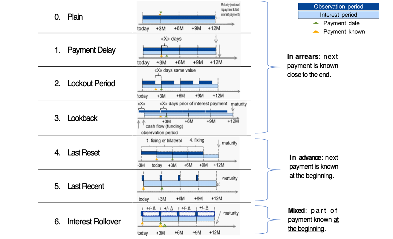
Figure 1: Overview of alternative techniques for calculating compounded SARON. Source: Financial Stability Board (2019).

0) Plain (in arrears): The observation period is identical to the interest period. The notional is paid at the start of the period and repaid on the last day of the contract period together with the last interest payment. Moreover, a Plain (in arrears) structure reflects the movement in interest rates over the full interest period and the payment is made on the day that it would naturally be due. On the other hand, given publication timing for most RFRs (T+1), the requiring payment is on the same day (T+1) that the final payment amount is known (T+1). An exception is SARON, as SARON is published one business day (T+0) before the overnight loan is repaid (T+1).

Example: the 1-month compounded SARON based on the Plain technique is like the example explained in the previous article, but has a different start date (1 February 2019). The resulting 1-month compounded SARON is equal to -0.7340% and it is known one day before the payment date (i.e. known on 28 February 2019).

1) Payment Delay (in arrears): Interest rate payments are delayed by X days after the end of an interest period. The idea is to provide more time for operational cash flow management. If X is set to 2 days, the cash flow of the loan matches the cash flow of most OIS swaps. This allows perfect hedging of the loan. On the other hand, the payment in the last period is due after the payback of the notional, which leads to a mismatch of cash flows and a potential increase in credit risk.

Example: the 1-month compounded SARON is equal to -0.7340% and like the one calculated using the Plain (in arrears) technique. The only difference is that the payment date shifts by X days, from 1 March 2019 to e.g. 4 March 2019. In this case X is equal to 3 days.

2) Lockout Period (in arrears): The RFR is no longer updated, i.e. frozen, for X days prior to the end of an interest rate period (lockout period). During this period, the RFR on the day prior to the start of the lockout is applied for the remaining days of the interest period. This technique is used for SOFR-based Floating Rate Notes (FRNs), where a lockout period of 2-5 days is mostly used in SOFR FRNs. Nevertheless, the calculation of the interest rate might be considered less transparent for clients and more complex for product providers to be implemented. It also results in interest rate risk that is difficult to hedge due to potential changes in the RFR during the lockout period. The longer the lockout period, the more difficult interest rate risk can be hedged during the lockout period.

Example: the 1-month compounded SARON with a lockout period equal to 3 days (i.e. X equals 3 days) is equal to -0.7337% and known 3 days in advance of the payment date.

3) Lookback (in arrears): The observation period for the interest rate calculation starts and ends X days prior to the interest period. Therefore, the interest payments can be calculated prior to the end of the interest period. This technique is predominately used for SONIA-based FRNs with a delay period of X equal to 5 days. An increase in interest rate risk due to changes in yield curve is observed over the lifetime of the product. This is expected to make it more difficult to hedge interest rate risk.

Example: assuming X is equal to 3 days, the 1-month compounded SARON would start in advance, on January 29, 2019 (i.e. today minus 3 days). This technique results in a compounded 1-month SARON equal to -0.7335%, known on 25 February 2019 and payable on 1 March 2019.

4) Last Reset (in advance): Interest payments are based on compounded RFR of the previous period. It is possible to ensure that the present value is equivalent to the Plain (in arrears) case, thanks to a constant mark-up added to the compounded RFR. The mark-up compensates the effects of the period shift over the full life of the product and can be priced by the OIS curve. In case of a decreasing yield curve, the mark-up would be negative. With this technique, the product is more complex, but the interest payments are known at the start of the interest period, as a LIBOR-based product. For this reason, the mark-up can be perceived as the price that a borrower is willing to pay due to the preference to know the next payment in advance.

Example: the interest rate payment on 1 March 2019 is already known at the start date and equal to -0.7328% (without mark-up).

5) Last Recent (in advance): A single RFR or a compounded RFR for a short number of days (e.g. 5 days) is applied for the entire interest period. Given the short observation period, the interest payment is already known in advance at the start of each interest period and due on the last day of that period. As a consequence, the volatility of a single RFR is higher than a compounded RFR. Therefore, interest rate risk cannot be properly hedged with currently existing derivatives instruments.

Example: a 5-day average is used to calculate the compounded SARON in advance. On the start date, the compounded SARON is equal to -0.7339% (known in advance) that will be paid on 1 March 2020.

6) Interest Rollover (hybrid): This technique combines a first payment (installment payment) known at the beginning of the interest rate period with an adjustment payment known at the end of the period. Like Last Recent (in advance), a single RFR or a compounded RFR for a short number of days is fixed for the whole interest period (installment payment known at the beginning). At the end of the period, an adjustment payment is calculated from the differential between the installment payment and the compounded RFR realized during the interest period. This adjustment payment is paid (by either party) at the end of the interest period (or a few days later) or rolled over into the payment for the next interest period. In short, part of the interest payment is known already at the start of the period. Early termination of contracts becomes more complex and a compensation mechanism is needed.

Example: similar to Last Recent (in advance), a 5-day compounded SARON can be considered as installment payment before the starting date. On the starting date, the 5-day compounded SARON rate is equal to -0.7339% and is known to be paid on 1 March 2019 (payment date). On the payment date, an adjustment payment is calculated as the delta between the realized 1-month compounded SARON, equal to -0.7340% based on Plain (in arrears), and -0.7339%.

There is a trade-off between knowing the cash flows in advance and the desire for a payment structure that is fully hedgeable against realized interest rate risk. Instruments in the derivatives market currently use ‘in arrears’ payment structures. As a result, the more the option used for a cash product deviates from ‘in arrears’, the less efficient the hedge for such a cash product will be. In order to use one or more of these options for cash products, operational cash management (infrastructure) systems need to be updated. For more details about the calculation of the compounded SARON using the alternative techniques, please refer to Table 1 and Table 2 in the Appendix I. The compounding formula used in the calculation is explained in the previous article.

Overall, market participants are recommended to consider and assess all the options above. Moreover, the financial institutions should individually define action plans with respect to their own product strategies.

Conclusions

The transition from IBOR to alternative reference rates affects all financial institutions from a wide operational perspective, including how products are created. Existing LIBOR-based cash products need to be replaced with SARON-based products as the mortgages contract. In the next installment, IBOR Reform in Switzerland – Part III, the latest information from the Swiss National Working Group (NWG) and market developments on the compounded SARON will be explained in more detail.

Appendix I – II

Contact

For more information about the challenges and latest developments on SARON, please contact Martijn Wycisk or Davide Mastromarco of Zanders’ Swiss office: +41 44 577 70 10.

The other articles on this subject: 

Transition from CHF LIBOR to SARON, IBOR Reform in Switzerland, Part I
Compounded SARON and Swiss Market Development, IBOR Reform in Switzerland, Part III
Fallback provisions as safety net, IBOR Reform in Switzerland, Part IV

References

1. Mastromarco, D. Transition from CHF LIBOR to SARON, IBOR Reform in Switzerland – Part I. February 2020.
2. National Working Group on Swiss Franc Reference Rates. Discussion paper on SARON Floating Rate Notes. July 2019.
3. National Working Group on Swiss Franc Reference Rates. Executive summary of the 12 November 2019 meeting of the National Working Group on Swiss Franc Reference Rates. Press release November 2019.
4. National Working Group on Swiss Franc Reference Rates. Starter pack: LIBOR transition in Switzerland. December 2019.
5. Financial Stability Board (FSB). Overnight Risk-Free Rates: A User’s Guide. June 2019.
6. ISDA. Supplement number 60 to the 2006 ISDA Definitions. October 2019.
7. ISDA. Interbank Offered Rate (IBOR) Fallbacks for 2006 ISDA Definitions. December 2019.
8. National Working Group on Swiss Franc Reference Rates. Executive summary of the 7 May 2020 meeting of the National Working Group on Swiss Franc Reference Rates. Press release May 2020

The standard model, as defined by IFRS 17, of measuring the value of insurance contracts is the ‘building blocks approach’. In this approach, the value of the contract is measured as the sum of the following components:

• Block 1: Sum of the future cash flows that relate directly to the fulfilment of the contractual  obligations.
• Block 2: Time value of the future cash flows. The discount rates used to determine the time value reflect the characteristics of the insurance contract.
• Block 3: Risk adjustment, representing the compensation that the insurer requires for bearing the uncertainty in the amount and timing of the cash flows.
• Block 4: Contractual service margin (CSM), representing the amount available for overhead and profit on the insurance contract. The purpose  of the CSM is to prevent a gain at initiation of the contract.

Risk adjustment vs risk margin

IFRS 17 does not provide full guidance on how the risk adjustment should be calculated. In theory, the compensation required by the insurer for bearing the risk of the contract would be equal to the cost of the needed capital. As most insurers within the IFRS jurisdiction capitalize based on Solvency II (SII) standards, it is likely that they will leverage on their past experience. In fact, there are many similarities between the risk adjustment and the SII risk margin.

The risk margin represents the compensation required for non-hedgeable risks by a third party that would take over the insurance liabilities. However, in practice, this is calculated using the capital models of the insurer itself. Therefore, it seems likely that the risk margin and risk adjustment will align. Differences can be expected though. For example, SII allows insurers to include operational risk in the risk margin, while this is not allowed under IFRS 17.

Liability adequacy test

Determining the impact of IFRS 17 is not straightforward: the current IFRS accounting standard leaves a lot of flexibility to determine the reserve value for insurance liabilities (one of the reasons for introducing IFRS 17). The reserve value reported under current IFRS is usually grandfathered from earlier accounting standards, such as Dutch GAAP. In general, these reserves can be defined as the present value of future benefits, where the technical interest rate and the assumptions for mortality are locked-in at pricing.

However, insurers are required to perform liability adequacy testing (LAT), where they compare the reserve values with the future cash flows calculated with ‘market consistent’ assumptions. As part of the market consistent valuation, insurers are allowed to include a compensation for bearing risk, such as the risk adjustment. Therefore, the biggest impact on the reserve value is expected from the introduction of the CSM.

The IASB has defined a hierarchy for the approach to measure the CSM at transition date. The preferred method is the ‘full retrospective application’. Under this approach, the insurer is required to measure the insurance contract as if the standard had always applied. Hence, the value of the insurance contract needs to be determined at the date of initial recognition and consecutive changes need to be determined all the way to transition date. This process is outlined in the following case study.

A case study

The impact of the new IFRS standards is analyzed for the following policy:

• The policy covers the risk that a mortgage owner deceases before the maturity of the loan. If this event occurs, the policy pays the remaining notional of the loan.
• The mortgage is issued on 31 December 2015 and has an initial notional value of € 200,000 that is amortized in 20 years. The interest percentage is set at 3 per cent.
• The policy pays an annual premium of € 150. The annual estimated costs of the policy are equal to 10 per cent of the premium.

In the case of this policy, an insurer needs to capitalize for the risk that the policy holder’s life expectancy decreases and the risk that expenses will increase (e.g. due to higher than expected inflation). We assume that the insurer applies the SII standard formula, where the total capital is the sum of the capital for the individual risk types, based on 99.5 per cent VaR approach, taking diversification into account.

The cost of capital would then be calculated as follows:

• Capital for mortality risk is based on an increase of 15 per cent of the mortality rates.
• Capital for expense risk is based on an increase of 10 per cent in expense amount combined with an increase of 1 per cent in the inflation.
• The diversification between these risk types is assumed to be 25 per cent.
• Future capital levels are assumed to be equal to the current capital levels, scaled for the decrease in outstanding policies and insurance coverage.
• The cost-of-capital rate equals 6 per cent.

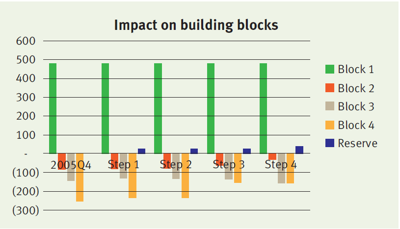
At initiation (i.e. 2015 Q4), the value of the contract under the new standards equals the sum of:

• Block 1: € 482
• Block 2: minus € 81
• Block 3: minus € 147
• Block 4: minus € 254

Consecutive changes

The insurer will measure the sum of blocks 1, 2 and 3 (which we refer to as the fulfilment cash flows) and the remaining amount of the CSM at each reporting date. The amounts typically change over time, in particular when expectations about future mortality and interest rates are updated. We distinguish four different factors that will lead to a change in the building blocks:

Step 1. Time effect
Over time, both the fulfilment cash flows and the CSM are fully amortized. The amortization profile of both components can be different, leading to a difference in the reserve value.

Step 2. Realized mortality is lower than expected
In our case study, the realized mortality is about 10 per cent lower than expected. This difference is recognized in P&L, leading to a higher profit in the first year. The effect on the fulfilment cash flows and CSM is limited. Consequently, the reserve value will remain roughly the same.

Step 3. Update of mortality assumptions
Updates of the mortality assumptions affect the fulfilment cash flows, which is simultaneously recognized in the CSM. The offset between the fulfilment cash flows and the CSM will lead to a very limited impact on the reserve value. In this case study, the update of the life table results in higher expected mortality and increased future cash outflows.

Step 4. Decrease in interest rates
Updates of the interest rate curve result in a change in the fulfilment cash flows. This change is not offset in the CSM, but is recognized in the other comprehensive income. Therefore a decrease in the discount curve will result in a significant change in the insurance liability. Our case study assumes a decrease in interest rates from 2 per cent to 1 per cent. As a result, the fulfilment cash flows increase, which is immediately reflected by an increase in the reserve value.

The impact of each step on the reserve value and underlying blocks is illustrated below.

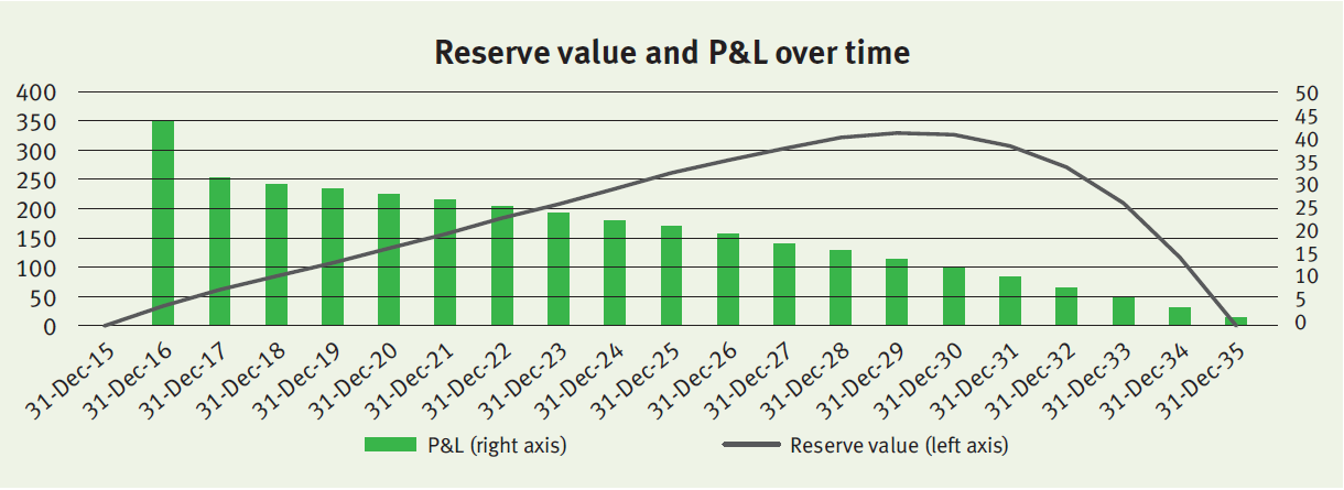
Onwards

The policy will evolve over time as expected, meaning that mortality will be realized as expected and discount rates do not change anymore. The reserve value and P&L over time will evolve as illustrated below.

The profit gradually decreases over time in line with the insurance coverage (i.e. outstanding notional of the mortgage). The relatively high profit in 2016 is (mainly) the result of the realized mortality that was lower than expected (step 2 described above).

As described before, under the full retrospective application, the insurer would be required to go all the way back to the initial recognition to measure the CSM and all consecutive changes. This would require insurers to deep-dive back into their policy administration systems. This has been acknowledged by the IASB by allowing insurers to implement the standards three years after final publication. Insurers will have to undertake a huge amount of operational effort and have already started with their impact analyses. In particular, the risk adjustment seems a challenging topic that requires an understanding of the capital models of the insurer.

Zanders can support in these qualitative analyses and can rely on its past experience with the implementation of Solvency II.

Solvency II aims to unify the EU insurance market and will come into effect on January 1st 2016. The technical specifications published by EIOPA will be used for interim reporting during 2015.

Although the specifications are not yet finalized, it is unlikely that they will change extensively. The technical specifications consist of two parts; part one focuses on the valuation and calculation of the capital requirements and part two focuses on the long-term guarantee (LTG) package. The LTG package was agreed upon in November 2013 and has been one of the key areas of debate in the Solvency II legislation.

Artificial volatility

The LTG package consists of regulatory measures to ensure that short-term market movements are appropriately treated with regards to the long-term nature of the insurance business. It aims to prevent ‘artificial’ volatility in the ‘own funds’ of insurers, while still reflecting the market consistent approach of Solvency II. When insurance companies invest long-term in fixed income markets, they are exposed to credit spread fluctuations not related to an increased probability of default of the counterparty.

These fluctuations impact the market value of the assets and own funds, but not the return of the investments itself as they are held to maturity. The LTG package consists of three options for insurers to deal with this so-called ‘artificial’ volatility: the Volatility Adjustment, the Matching Adjustment and transitional measures.

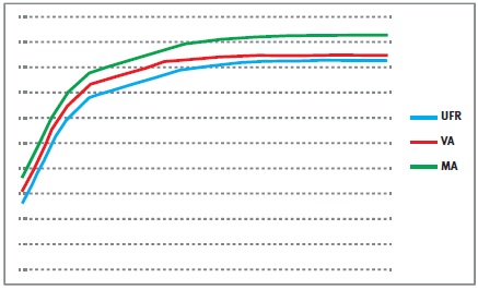
Figure 1

The transitional measures allow insurers to move smoothly from Solvency I to Solvency II and apply to the risk-free curve and technical provisions. However, the most interesting measures are the Volatility Adjustment and the Matching Adjustment. The impact of both measures is difficult to assess and it is a strategic choice which measure should be applied.

Both try to prevent fluctuations in the own funds due to artificial volatility, yet their requirements and use are rather different. To find out more about these differences, we immersed ourselves into the impact of the Volatility Adjustment and the Matching Adjustment.

The Volatility Adjustment

The Volatility Adjustment (VA) is a constant addition to the risk-free curve, which used to calculate the Ultimate Forward Rate (UFR). It is designed to protect insurers with long-term liabilities from the impact of volatility on the insurers’ solvency position. The VA is based on a risk-corrected spread on the assets in a reference portfolio. It is defined as the spread between the interest rate of the assets in the reference portfolio and the corresponding risk-free rate, minus the fundamental spread (which represents default or downgrade risk).

The VA is provided and updated by EIOPA and can differ for each major currency and country. The VA is added to the liquid part of the risk-free zero-coupon rates, i.e. until the so-called Last Liquid Point (LLP). After the LLP, the curve converges to the UFR. The resulting rates are used to produce the relevant risk-free curve.

The Matching Adjustment

The Matching Adjustment (MA) is a parallel shift applied to the entire basic risk-free term structure and serves the same purpose as the VA. The MA is calculated based on the match between the insurers’ assets and the liabilities. The MA is corrected for the fundamental spread. Note that, although the MA is usually higher than the VA, the MA can possibly become negative. The MA can only be applied to a portfolio of life insurance obligations with an assigned portfolio of assets that covers the best estimate of the liabilities.

The mismatch between the cash flows of the assets and the cash flows of the liabilities must not be a material risk in relation to the risks inherent to the insurance business. These portfolios need to be identified, organized and managed separately from other activities of the insurers. Furthermore, the assigned portfolio of assets cannot be used to cover losses arising from other activities of the insurers.

The more of these portfolios are created for an insurance company, the less diversification benefits are possible. Therefore, the MA does not necessarily lead to an overall benefit.

Differences between VA and MA

The main difference between the VA and the MA is that the VA is provided by EIOPA and based on a reference portfolio, while the MA is based on a portfolio of the insurance company.

Other differences include:

• The VA is applied until the LLP, after which the curve converges to the UFR, while the MA is a parallel shift of the whole risk-free curve;
• The MA can only be applied to specifically identified portfolios;
• The VA can be used together with the transitional measures in the preparatory phase, the MA cannot;
• The MA has to be taken into account for the calculation of the Solvency Capital Requirement (SCR) for spread risk. The VA does not respond to SCR shocks for spread risks.

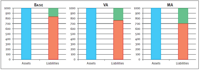
Figure 2: Graphical representations of balance sheets. The blue box represents the assets, the red box the liabilities, and the green box the available capital.

The impact of the VA and MA is twofold. Both adjustments have a direct impact on the available capital and next to this, the MA impacts the SCR. As a result, the level of free capital is affected as well. While the exact impact of the adjustments depends on firm-specific aspects (e.g. cash flows, the asset mix), an indication of the effects on available capital as well as the SCR is given in Figure 2. Please note that this is an example in which all numbers are fictitious and used merely for illustrative purposes.

Impact on available capital

Both the VA and the MA are an addition to the curve used to discount the liabilities, and will therefore lead to an increase in the available capital. The left chart in Figure 2 shows the Base scenario, without adjustment to the risk-free curve. Implementing the VA reduces the market value of the liabilities, but has no effect on the assets. As a result, the available capital increases, which can be seen in the middle chart.

A similar but larger effect can be seen in the right chart, which displays the outcome of the MA. The larger effect on the available capital after the MA compared to the VA is due to two components.

1. The MA is usually higher than the VA, and
2. the MA is applied to the whole curve.

Impact on the SCR

The calculation of the total SCR, using the Standard Formula, depends on several marginal SCRs. These marginal SCRs all represent a change in an associated risk factor (e.g. spread shocks, curve shifts), and can be seen as the decrease in available capital after an adverse scenario occurs. The risk factors can have an impact on assets, liabilities and available capital, and therefore on the required capital.

Take for example the marginal SCR for spread risk. A spread shock will have a direct, and equal, negative impact on the assets for each scenario. However, since a change in the assets has an impact on the level of the MA, the liabilities are impacted too when the MA is applied. The two left charts in Figure 3 show the results of an increase in the spread, where, by applying the spread shock, the available capital decreases by the same amount (denoted by the striped boxes).

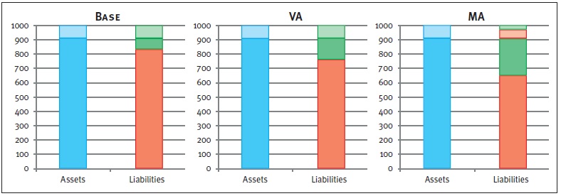
Figure 3: Graphical representations of balance sheets after a positive spread shock. The lined boxes represent a decrease of the corresponding balance sheet item. Note that, in the MA case, the liabilities decrease (striped red box) due to an increase of the MA.

Hence, the marginal SCR for the spread shock will be equal for the Base case and the VA case. The right chart displays an equal effect on the assets. However, the decrease of the assets results in an increase of the MA. Therefore, the liabilities decrease in value too. Consequently, the available capital is reduced to a lesser extent compared to the Base or VA case.

The marginal SCR example for a spread shock clearly shows the difference in impact on the marginal SCR between the MA on the one hand, and the VA and Base case on the other hand. When looking at marginal SCRs driven by other risk factors, a similar effect will occur. Note that the total SCR is based on the marginal SCRs, including diversification effects. Therefore, the impact on the total SCR differs from the sum of the impacts on the marginal SCRs.

Impact on free capital

The impact on the level of free capital also becomes clear in Figure 3. Note that the level of free capital is calculated as available capital minus required capital. It follows directly that the application of either the VA or the MA will result in a higher level of free capital compared to the Base case. Both adjustments initially result in a higher level of available capital.

In addition, the MA may lead to a decrease in the SCR which has an extra positive impact on the free capital. The level of free capital is represented by the solid green boxes in Figure 3. This figure shows that the highest level of free capital is obtained for the MA, followed by the VA and the Base case respectively.

Conclusion

Our example shows that both the VA and the MA have a positive effect on the available capital. Apart from its restrictions and difficulties of the implementation, the MA leads to the greatest benefits in terms of available and free capital.

In addition, applying the MA could lead to a reduction of the SCR. However, the specific portfolio requirements, practical difficulties, lower diversification effects and the possibility of having a negative MA, could offset these benefits.

Besides this, the MA cannot be used in combination with the transitional measures. In order to assess the impact of both measures on the regulatory solvency position for an insurance company, an in-depth investigation is required where all firm specific characteristics are taken into account.

The introduction of the UFR was an attempt to address three problems. Firstly, as interest rates currently stand, applying the UFR has the effect of increasing rates with a maturity of 20 years or more (see figure 1). This causes the present value of long-term liabilities to fall, which means funding ratios and capital ratios rise. Secondly, the interest rate market for long maturities is assumed to be insufficiently liquid to permit a reliable market valuation, which means the value of liabilities may be very volatile.

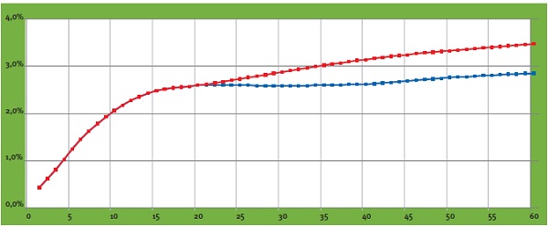
Figure 1: Spot yield curve with UFR (red) and without UFR (blue) as of September 30, 2013

The third problem addressed by the UFR is the desire to escape the vicious circle which is created when interest rate risks are hedged. Due to demand among pension funds and insurers for swaps with long maturities, these interest rates are falling, necessitating further interest rate hedging and triggering a renewed rise in demand.

Risk management

The UFR, however, is raising questions about risk management by insurers and pension funds, who are required to use the UFR when valuing their liabilities in their regulatory reports. From a risk management perspective, however, there are important arguments against hedging interest rate risks on the basis of the UFR.

The UFR is not an economic reality: there are no instruments on the market which generate the same returns as the UFR-adjusted interest rates. Consequently, there is an imbalance between the value as reported to DNB and the available instruments on the market for managing the risks. Furthermore, the UFR is only applied to the liabilities on the balance sheet, and not to the assets. This creates a discrepancy between the economic reality of the assets and the ‘paper’ UFR reality of the liabilities. If a company’s assets and liabilities have identical interest rate profiles, the company does not run an interest rate risk; nonetheless, its UFR-based funding ratio does change in line with interest rate movements on the market. There is also greater interest rate sensitivity around the 20-year interest rate point: past this point, market interest rates are partially or entirely disregarded. Lastly, there is a political risk (which cannot be hedged) that the UFR method may be revised by the regulator – a fact underlined by recent developments.

Insurers and pension funds are compelled to keep two different sets of records: a ‘UFR report’ for the regulator and an economic version on which the interest rate risk is actually managed. Both records have their own, specific risks.

Insurers: debate and uncertainty

Understandably, the UFR has created quite a furor among insurers. In June 2013, EIOPA published the results of a survey of insurers who offer long-term guarantee products. Interestingly, EIOPA acknowledges in this publication that the UFR entails significant risks. Potentially, the UFR could mislead regulators, meaning that any action is taken too late. Moreover, the design of the UFR – specifically, the speed at which the forward rate converges towards the UFR – has long been a source of uncertainty. EIOPA advises using what is known as the ‘20+40’ convergence (whereby market interest rates are used up to and including 20 years and, 40 years later, the forward rate has converged to the UFR). Both insurers and the European Parliament, however, are pressing for a switch to a ‘20+10’ convergence.

Proponents of this shorter convergence period point to the lower sensitivity to shocks in (long-term) market interest rates, which would help stabilize the valuation of liabilities. One drawback of a short convergence period is the increased volatility of own funds. This is because the assets are discounted at market interest rates and are sensitive to changes in interest rates, whereas the liabilities are not. Moreover, the potential impact of a change in the level of the UFR is greater when the convergence period is shorter.

While the debate continues among European insurers, DNB has already compelled Dutch insurers to use the UFR. In so doing, DNB is largely taking its cue from EIOPA’s latest advice. However, there is a high risk that the convergence period will change in the definitive Solvency II legislation, meaning that, eventually, insurers will have to switch to a different UFR.

Pensions: DNB is pursuing its own course

The UFR committee
In October 2013, the UFR committee advised the Dutch cabinet to abandon the current method for pension funds, which involves a fixed UFR of 4.2%. The committee advises using the UFR as an ultimate rate, based on the average forward rates of the last 120 months, with an infinite convergence period.

The UFR will then become a moving target based on current market rates. As things currently stand, this would mean a UFR of 3.9% – which is significantly different to the current UFR.

The cabinet informed the UFR committee in a response that the recommendation of applying a moving target UFR will be implemented from 2015 onwards. This will only accentuate the contrast between Europe and the Dutch pension landscape. In addition to an economic report and the current UFR report, it will compel pension funds to also prepare an adjusted UFR report for 2015.

The situation as regards pension funds illustrates the political risk. Following criticism in Dutch academic circles about the high sensitivity affecting the 20-year forward rate, DNB adapted the rules specifically for pension funds. These funds must now continue applying the forward rate past the 20-year point (with fixed weightings) and the spot rates are averaged over the last three months.

Since then, in its advisory report, the UFR committee has proposed a completely new calculation method (see insert), which may have a big impact on funding ratios. It is not inconceivable that, if the yield curve fluctuates significantly, the UFR will yet again be changed. In addition, there are also long-term risks to be taken into account. The UFR could potentially create discrepancies between the pension entitlements of current and future pensioners.

The higher funding ratio resulting from the application of the UFR reduces the likelihood of increases in contributions and cuts to pensions at the present time – which is an advantage for current pensioners. If, however, the yield turns out lower than assumed, future pensioners will have fewer funds at their disposal. Potentially, therefore, pension rights may end up being transferred from younger to older generations.

Conclusion

The EIOPA study and the UFR committee illustrate that the introduction of the UFR has made the world of insurance more complex. In risk management terms, it has created two landscapes and it is not yet clear exactly what the UFR landscape will look like. From an economic perspective, the majority of risk managers will give priority to hedging risks. To prevent interference by the regulator, however, the UFR value must always be closely monitored. Furthermore, the impending change to the UFR method for pension funds reaffirms that the political risk is a significant, unmanageable factor.