Executive Summary

RMA will be an optional model within IFRS 9 for net interest rate repricing risk¹ in dynamic, open portfolios (for example, where new deposits or loans are continually added and existing positions mature or reprice). The IASB also proposes withdrawing the IAS 39 macro hedge requirements (and the IFRS 9 option to apply them) and adding related IFRS 7 disclosures.

Compared with current IFRS 9 hedge accounting, RMA shifts from item-level hedges to portfolio net-position accounting, better aligned to typical banking book features (for example, non-maturity deposits and pipeline exposures). Compared with IAS 39 macro hedging (including the EU carve-out), it replaces bucket-based rules and carve-out reliefs with a principles-based net exposure model.

At a high level, the RMA model works as follows:

• Set the target: the entity specifies how much net interest rate risk it aims to mitigate over time, within defined risk limits and not exceeding the net exposure in each time band (bucket). The target can be updated prospectively as the balance sheet evolves.
• Link to derivatives: external interest rate derivatives can be designated. The model uses benchmark derivatives (hypothetical instruments with zero fair value at inception) to represent the risk the entity intends to mitigate.
• Recognize an adjustment: a risk mitigation adjustment is recognized on the balance sheet. It equals the lower of (I) the cumulative value change of the designated derivatives and (II) the cumulative value change of the benchmark derivatives. Any remaining derivative gains or losses (and any ‘excess’ adjustment) go to profit or loss.
• Release to earnings: the risk mitigation adjustment is released to profit or loss as the underlying repricing effects occur.

RMA is a meaningful step toward aligning accounting with how banks manage banking-book interest rate risk in dynamic, open portfolios. At the same time, the ED leaves important practical questions open, notably on benchmark-derivative construction, operation of the excess test, and the level of data, systems, and governance needed for ongoing application.

After the 31 July 2026 deadline, the IASB will review comment letters and fieldwork feedback and decide whether further deliberations are needed, so finalization is likely to take several years. Even once the IASB issues a final standard, application in the EU would still depend on completion of the endorsement process (EFRAG advice, Commission adoption, and Parliament/Council scrutiny).

Introduction

On December 3^rd, 2025, the IASB published the ED proposing RMA for interest rate risk in dynamic portfolios. RMA is the result of the IASB’s long-running efforts on accounting for dynamic interest rate risk management, previously referred to as DRM. RMA focuses on repricing risk, which is the interest rate risk that arises when the timing and amount of repricing differ between assets and liabilities.

The aim is to better reflect how banks manage interest rate risk in the banking book at a portfolio level, an area where existing hedge accounting requirements have long been seen as difficult to apply in a way that aligns with real-world balance sheet management.

The IASB presents RMA as a step forward, to better reflect how banks manage interest rate risk in the banking book at a portfolio level, an area in which existing IAS 39 and IFRS 9 hedge accounting requirements have long been viewed as difficult to apply in a way that aligns with real-world, dynamic balance sheet management. In the IASB’s view, RMA is intended to improve that alignment, increase transparency about the effects of repricing-risk management on future cash flows, strengthen consistency between what is managed and what is eligible for accounting treatment, and recognize in the financial statements the extent to which repricing risk has actually been mitigated and the related economic effects.

This article provides a structured overview of the proposed RMA model and its key mechanics. Throughout the article, Zanders provides practical insights on the impact on entities, highlighting the key areas that will shape implementation challenges and accounting results. These insights draw on Zanders' 2025 survey on interest rate risk management and hedge accounting, as well as analysis of stakeholder feedback such as EFRAG's draft comment letter². The practical implications will depend in part on the outcome of field testing.

Overview of RMA

The model components and their relationships are presented in Figure 1 below:

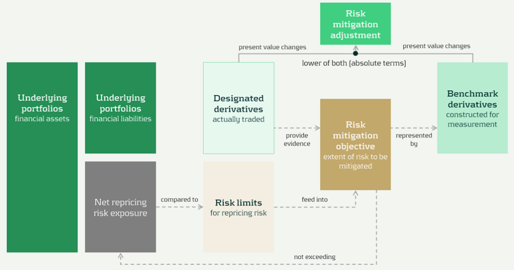
Figure 1: RMA model component overview (source: IASB ED – Snapshot, December 2025)

The RMA model is built around a small set of linked building blocks that start with the bank’s balance-sheet exposures and end with the accounting adjustment that reflects risk management in the financial statements:

• Underlying portfolios: the managed portfolios that expose the entity to repricing risk.
• Net repricing risk exposure: the net position created by the interaction of asset and liability repricing profiles (i.e., the aggregate repricing mismatch the bank is exposed to).
• Risk limits: the bank’s risk appetite and constraints for the managed exposure. In the model, these limits act as an important boundary.
• Risk mitigation objective: the clearly articulated target for how much of the net repricing risk exposure management intends to mitigate (within risk limits). This objective is the central anchor in the model.
• Designated derivatives: the derivatives the bank trades to achieve the risk mitigation objective.
• Benchmark derivatives: hypothetical derivatives constructed to represent the risk mitigation objective for measurement purposes. They translate the objective into a measurable reference profile against which fair value changes can be assessed.
• Risk mitigation adjustment: the accounting output of the model, which is the lower of the change in fair value of the benchmark derivatives and the designated derivatives (in absolute terms).

The section headers contain the relevant paragraph of the ED. The body of the text refers to the ED amendments to IFRS 9 [7.x.), application guidance [B7.x.x), basis for conclusions [BCx), and illustrative examples [IEx), and amendments to IFRS 7 [30x).

Speak to a Zanders expert

Objective and scope [ED 7.1]

IFRS 9 hedge accounting improves alignment for many strategies, but it does not fully capture dynamic, open-portfolio (macro) management of banking book repricing risk—where entities manage interest rate risk of net open positions rather than hedging individual instruments. The RMA model is intended to reflect this more directly and reduce reliance on proxy hedges that can obscure transparency and comparability.

The objective and scope of RMA can be summarized as follows:

• Objective: RMA is, like current hedge accounting under IAS 39 and IFRS 9, an optional model within IFRS 9. The objective is to reflect the economic effect of risk management activities and improve transparency by explaining why and how derivatives are used to mitigate repricing risk and how effectively they do so —bringing reporting closer to actual interest rate risk management practices [7.1.3]. It is the IASB’s intention to withdraw the requirements in IAS 39 for macro hedge accounting and the option in paragraph 6.1.3 of IFRS 9 to apply the requirements in IAS 39 to a portfolio hedge of interest rate risk.
• Scope/eligibility: An entity may apply RMA if, and only if, all of the following are met [7.1.4]:
  • Business activities give rise to repricing risk through the recognition and derecognition of financial instruments that expose the entity to repricing risk.The risk management strategy specifies risk limits within which repricing risk, based on a mitigated rate, is to be mitigated, including the time bands and frequency.
  • The entity mitigates repricing risk arising from underlying portfolios on a net basis using derivatives, consistent with the entity’s risk management strategy.
• Application discipline: RMA is applied at the level where repricing risk is actually managed and requires robust formal documentation (strategy, mitigated rate, mitigated time horizon, risk limits, and methods for determining exposures and benchmark derivatives) [7.1.6, 7.1.7].

Key considerations and insights

1. Objective: RMA’s objective to reflect the economic effect of risk management activities may not always coincide with eliminating accounting mismatches (as suggested by other key considerations and insights later in this article). For example, EFRAG’s draft comment letter agrees that faithful representation is a key objective and could improve current accounting, for example, by reducing reliance on proxy hedging. However, it questions whether this should be treated as equally important as eliminating accounting mismatches. This aligns with the concerns expressed around the impact on the hedge effectiveness by several European banks in Zanders’ 2025 survey on interest rate risk management and hedge accounting3, while more than 80% of the participants assessed its effectiveness under the current hedge accounting approach as acceptable.

Net repricing risk exposure [ED 7.2]

Entities are required to determine a net repricing risk exposure across underlying portfolios by aggregating repricing risk exposure using expected repricing dates, within each repricing time band as required to be defined in formal documentation.

Key requirements include:

• Eligible items Underlying portfolios can include [7.2.1; B7.2.1–B7.2.2]:
  • Financial assets measured at amortized cost or FVOCI,
  • Financial liabilities at amortized cost, and,
  • Eligible future transactions that may result in recognition/derecognition of such items.
• Portfolio view and behavioral profiles: Items that may not show sensitivity on an individual basis (for example, demand deposits) can still contribute to repricing risk on a portfolio basis. A stable ‘core’ portion may be treated as behaving like longer-term funding if supported by reasonable and supportable assumptions and consistent with risk management [B7.2.2].
• Expected repricing dates and time bands: Expected repricing dates must be measured reliably using reasonable and supportable information (including behavioral characteristics such as prepayments and deposit stability). Time bands and risk measures (e.g., maturity gap or PV01) must be consistent with actual risk management [7.2.5–7.2.9; B7.2.10–B7.2.16].
• Equity modeling as a proxy: Own equity is not eligible for inclusion in underlying portfolios, but the model acknowledges that some entities assess repricing risk from cash/highly liquid variable-rate assets only to the extent they are ‘funded by equity’. If internal equity modeling (e.g., replicating portfolios) is used for risk management, it can serve as a proxy to determine how much of those exposures are included in net repricing risk exposure [B7.2.17; IE184-IE191].

Key considerations and insights

2. Eligibility: RMA aims to reflect net repricing risk management, but eligibility rules can make the net repricing risk exposure only a partial proxy for the position Treasury actually manages. For example, banks might include fair value through profit or loss (FVTPL) items for interest rate risk management but these are not allowed as underlying items in the net repricing risk exposure (also noted by EFRAG).

3. Risk management by time bands (1/2): RMA requires a risk mitigation objective based on the net repricing risk exposure determined for each repricing time band, but it is unclear how entities that do not manage their interest rate risk across time bands would then apply the RMA model, as noted by EFRAG.

4. Risk management by time bands (1/2): RMA requires the same risk measure (e.g., maturity gap or PV01) for all exposures within each repricing time band [B7.2.13], but banks’ risk management practice might deviate from this.

5. Equity treatment: RMA introduces an equity proxy approach that allows partial inclusion of variable-rate assets based on modelled equity, viewing equity as residual and ineligible for direct inclusion. This is an addition compared to the DRM staff papers. Banks' risk management practices might treat equity differently (e.g., by modeling it).

Designated derivatives [ED 7.3]

Under RMA, banks can designate external derivatives (e.g., interest rate swaps, forwards, futures, options) used to manage net repricing risk as hedging instruments. Eligible derivatives are generally consistent with IFRS 9. All designated derivatives collectively mitigate the net portfolio risk and remain recognized at fair value.

Eligibility depends on the following items:

• Mitigation: Derivatives can only be designated to the extent that they mitigate the net repricing risk exposure [7.3.6].
• External counterparty: Derivatives must be with a counterparty external to the reporting entity. Intragroup derivatives may qualify only in the separate or individual financial statements of the relevant entities, and are not eligible in the consolidated financial statements of the group [7.3.4].
• Designate once: Derivatives already in a hedging relationship for interest rate risk in accordance with Chapter 6 of IFRS 9 are not eligible [7.3.5].
• Options: Written options are generally excluded, unless part of a net written option position that offsets a purchased option, resulting in a net purchased position overall [7.3.2(a), 7.3.3].

Banks can designate derivatives in full or in part (e.g., designating 80% of a swap if only that portion manages interest rate risk), but the selected portion must align with the documented risk mitigation objective.

Once derivatives are designated, they can only be removed from RMA if they are no longer held to mitigate the net repricing risk exposure under the entity’s risk management strategy.

Key considerations and insights

As the EFRAG comment letter notes: 6. Options and off-market derivatives: Further guidance is needed on how to treat options (for example, time value) and off-market derivatives (non-zero initial fair value) within the designation mechanics.

7. De-designation: The ED does not allow voluntary de-designation, but banks often manage changes by entering into offsetting trades rather than settling existing positions.

Risk mitigation objective [ED 7.4]

The risk mitigation objective is the bridge between risk mitigation intent and what’s actually executed: it sets how much net repricing risk exposure the entity aims to mitigate within risk limits [7.4.2]. The benchmark derivatives and consequently the risk mitigation adjustment are built from this risk mitigation objective (see next sections), enabling partial hedging while avoiding objectives that aren’t supported by actual designated hedges. [ED 7.4.1, B7.4.2–B7.4.3].

Key requirements:

• Evidence-based: The objective must be consistent with the repricing risk mitigated by designated derivatives—it’s a matter of fact, not a free choice. [ED 7.4.1, B7.4.2–B7.4.3]
• Absolute, not proportional: It’s stated as an absolute amount of risk (e.g., PV01), not ‘X% of each instrument’ [B7.4.2].
• Capped by exposure: It cannot exceed net repricing risk exposure (overhedge) in any time band [7.4.1, B7.4.2–B7.4.3].
• Measurement basis: The risk mitigation objective should be set using the same risk measure (e.g., DV01) used to quantify exposure [ED B7.4.1].

Key considerations and insights

8. Repricing time bands are a key design choice: the risk mitigation objective is specified and capped by the net repricing risk exposure in each time band. Executing (and designating) hedges in neighboring tenors (a common practice) can create residual P&L volatility, because only the portion aligned to that time band’s net repricing risk exposure is reflected in the risk mitigation adjustment.

9. Degree of freedom risk limits: While RMA imposes strict alignment requirements between net repricing risk exposure, risk mitigation objective, and designated derivatives on measures and time bands, entities retain strategic flexibility on risk limits. Risk limits do not need to be specified per time band [B7.4.6], allowing entities to set overarching frameworks rather than granular constraints.

Benchmark derivatives [ED 7.4]

Benchmark derivatives are introduced to measure hedge performance: modelled (hypothetical) derivatives that are not executed and not recognized on the balance sheet, but are constructed to replicate the timing and amount of repricing risk captured in the risk mitigation objective, as presented in Figure 1 above and Figure 2 below.

In practice, the benchmark derivative is designed to mirror the bank’s target risk position (e.g., a swap profile that matches the repricing ‘gap’ being mitigated), so its fair value movement represents how the net repricing risk exposure would change when interest rates move. If an entity intends to mitigate 70 of the 100 units of repricing risk in the 9-year time band by a 10-year swap, the benchmark derivative is based on 70 units and 9 year maturity [B7.4.8].

Benchmark derivatives should have an initial fair value of zero based on the mitigated rate [7.4.5]. These benchmark derivatives are therefore similar to the hypothetical derivative used in cash flow hedging [B6.5.5–B6.5.6 of IFRS 9].

Key considerations and insights

10. Operational burden (1/3) – benchmark derivatives: RMA intentionally separates designated derivatives from benchmark derivatives (constructed to start at zero fair value at the mitigated rate), so they won’t always share the same terms. This can become operationally heavy, as also noted by EFRAG.

Risk mitigation adjustment [ED 7.4]

The risk mitigation adjustment is the accounting output of the model and is presented as a single line item on the balance sheet (asset or liability). At each reporting date (so not necessarily the hedging date), the entity compares the cumulative fair value change of all designated derivatives with the cumulative fair value change of all the benchmark derivatives, and recognizes the lower of those two amounts (in absolute terms) [7.4.8] as the risk mitigation adjustment. That balance sheet adjustment is the mechanism that offsets the designated derivatives’ fair value changes in profit or loss; any remaining gain or loss (i.e., the portion not captured by the lower-of) is recognized directly in profit or loss as residual volatility/ineffectiveness [7.4.9].  This is visualized in Figure 2 below.

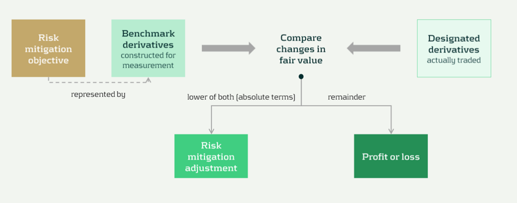
Figure 2 Recognition and measurement of risk mitigation adjustment (source: IASB ED – Snapshot, December 2025)

The 'lower of' mechanism ensures the risk mitigation adjustment never exceeds what's actually supported by either (I) the designated derivatives or (ii) the net exposure being hedged. This prevents over-recognition of hedging effects.

The risk mitigation adjustment is then recognized in profit or loss over time on a systematic basis that follows the repricing profile of the underlying portfolios [7.4.10], so the hedging effect shows up in the same periods in which the hedged repricing differences affect earnings.

Key considerations and insights

11. Operational burden (2/3) – risk mitigation adjustment: Heavy tracking requirements (including effects of settling vs offsetting trades), unclear calculation granularity, and complexity over time as the risk mitigation adjustment can flip between debit and credit, as noted by EFRAG.

12. RMA as a balance sheet item: The RMA model creates a separate balance sheet asset/liability (unlike current hedge accounting that adjusts hedged items or uses equity), introducing uncertainty around whether this item will attract RWA or require capital deductions until regulators provide guidance.

Prospective (RMA excess) and retrospective (unexpected changes) testing [ED 7.4]

RMA is designed to keep the accounting mechanics anchored to the net repricing risk exposure that actually remains in the underlying portfolios over time. Two tests can lead to changes to the risk mitigation adjustment. These tests are visualized in Figure 3 below, indicated by ① and ②.

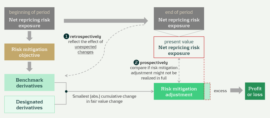
Figure 3 Risk mitigation adjustment and prospective and retrospective testing (source: IASB ED – Snapshot, December 2025)

The two tests are:

1. Benchmark adjustments for unexpected changes (retrospectively): First, benchmark derivatives must be adjusted when unexpected changes in the underlying portfolios reduce the net repricing risk exposure below the risk mitigation objective in a repricing time band (i.e., correction of overhedge), as they would otherwise no longer represent the repricing risk specified in the risk mitigation objective [7.4.6, B7.4.10].
2. Excess test to prevent unrealizable adjustments (prospectively): Second, an explicit excess assessment to prevent the risk mitigation adjustment from accumulating beyond what can be supported by the remaining net repricing risk exposure. If there is an indication that the accumulated risk mitigation adjustment may not be realized in full, the entity compares the risk mitigation adjustment to the present value of the net repricing risk exposure at the reporting date (discounted at the mitigated rate) [7.4.11–7.4.13]. This would happen if unexpected changes have not been fully reflected in the adjustments to the benchmark derivatives.

Any excess is recognized immediately in profit or loss by reducing the risk mitigation adjustment, and it cannot be reversed [7.4.14; BC101–BC103]. It acts like a safeguard: if revised behavioral assumptions shrink future repricing exposure, the unearned portion of the adjustment is released to P&L straight away.

Key considerations and insights

13. Operational burden (3/3) – benchmark derivatives: The reliance on ‘unexpected changes’ and time-band caps may force highly granular, frequently re-constructed benchmark derivatives, creating a mismatch versus designated derivatives. This could be operationally heavy, as noted by EFRAG.

14. Unclear testing and adjustment mechanics: The ‘excess’ framework is under-specified. Triggers and documentation expectations are unclear, and the present value test for net exposure is conceptually and operationally challenging, especially for modelled items (e.g., NMDs), as noted by EFRAG.

Discontinuation [ED 7.5]

Discontinuation is intentionally rare. RMA is not switched off because hedging activity changes. It only stops when the risk management strategy changes, and it stops prospectively from the date of change.

Key requirements include:

• Strategy: strategy triggers a change; activity does not. A change in how repricing risk is managed, such as changing the mitigated rate, changing the level at which repricing risk is managed (group vs entity), or changing the mitigated time horizon [7.5.1, 7.5.2].
• Prospective application: discontinue from the date the strategy change is made. No restatement of prior periods [7.5.1].

After discontinuation, the existing balance is recognized in profit or loss, either:

• Over time, on a systematic basis aligned to the repricing profile, if repricing differences are still expected to affect profit or loss [7.5.3(a)], or,
• Immediately if those repricing differences are no longer expected to affect profit or loss [7.5.3(b)].

Disclosures [IFRS 7]

The disclosures are meant to show, in a compact way, what risk is being mitigated, what derivatives are used, and what the model produced in the financial statements.

Key disclosures include:

• RMA balance sheet and P&L: risk mitigation adjustment closing balance and current-period P&L impact [30E].
• Risk strategy and exposure: repricing risk managed, portfolios in scope, mitigated rate and horizon, risk measure, and exposure profile [30H–30L].
• Designated derivatives: timing profile and key terms, notional amounts, carrying amounts, and line items, and FV change used in measuring the adjustment [30I, 30M].
• Sensitivity: effect of reasonably possible changes in the mitigated rate [30J].
  Volatility and roll-forward: FV changes not captured and where presented, plus reconciliation including excess amounts and discontinued balances [30N–30P].

Key considerations and insights

15- More, and more sensitive, disclosures: RMA adds extensive requirements (profiles, sensitivities, roll-forwards) that may reveal non-public positioning, so aggregation and materiality judgment matter.

Conclusions

The RMA proposal appears to be a constructive development toward reflecting the management of interest rate risk in dynamic portfolios more faithfully in financial reporting. Compared with existing approaches, it offers a clearer conceptual link between net repricing-risk management and accounting outcomes.

At the same time, several core mechanics might prove challenging in practice. In particular, further clarification would be helpful on the benchmark-derivative mechanism, the operation and trigger logic of the excess test, and the level of granularity and governance expected for the ongoing application. These areas will likely be central to implementation efforts, earnings volatility outcomes, and cross-bank comparability.
At this stage, practical outcomes may therefore differ significantly depending on interpretation and system design choices. Additional IASB guidance, informed by field testing and stakeholder feedback, could reduce that uncertainty and support more consistent application. Overall, RMA can be seen as a promising direction that improves conceptual alignment with risk management, while still requiring further clarification before its operational and reporting implications are fully settled.

We’ve spoken to many banks recently, and the message is clear: developing and implementing a climate reverse stress testing (RST) framework will be a significant challenge, particularly as it is a completely new regulatory expectation for climate risk from the PRA. Most banks are already familiar with RST in the context of credit, market, and liquidity risks. But extending this practice to climate introduces a different level of complexity.  

Until now, climate quantitative analysis has centered on standard stress testing and scenario analysis, asking what could happen under different climate pathways. Reverse stress testing flips the question: what climate pathway could push your business model to the point of failure?

You may have already fallen into the trap of believing these common myths; if so, it’s time to rethink your position: 

• “Our institution is not exposed to climate risk.” The PRA is unlikely to accept this - climate risk is systemic. It manifests as transition risk (such as carbon taxes or shifts in consumer expectations) and physical risk (both acute climate events and chronic changes). These drivers affect almost every portfolio: credit exposures like commercial loans and mortgages, market positions in bonds and equities, and even operational resilience. Hence, it is highly likely that your institution is already exposed to climate risk factors, directly or indirectly. 

• “Rain alone could never cause us to fail.” This could be true if it weren’t for the fact that risks don’t occur in isolation. Rainfall, carbon prices, GDP slowdown, and interest rate rises can interact in complex and non-linear ways to push an institution towards failure. Although a single risk factor might need to reach an extreme tail event to cause failure, multiple risk factors acting together don’t need to be extreme to push a firm to the brink. Plausible domino effects can occur - for example, in a mortgage portfolio, heavier rainfall increases flood risk, lowering property values and weakening collateral. At the same time, a rise in carbon prices lifts household energy bills, cutting disposable income and pushing up default probabilities. Higher PDs, combined with weaker collateral driving LGDs higher, can accelerate capital erosion towards the failure point.

• “The failure points are so extreme, there’s no benefit in analyzing them.” A failure point doesn’t have to mean the bank has collapsed entirely. In practice, it could be something completely plausible, such as the CET1 falling below 11% or liquidity buffers dropping under regulatory requirements. These are thresholds that banks already monitor as part of business-as-usual.  

• “What’s the benefit of RST? We already run standard stress tests.” RST forces firms to confront and explore extreme, and yet plausible, critical scenarios they might otherwise avoid. It can uncover vulnerabilities that remain hidden in conventional stress testing. 

We recommend that you should prepare for the following key challenges: 

• Defining failure points: Deciding exactly what a failure would look like is not straightforward and is the first challenge. Most firms will base the breaking point on a regulatory capital measure such as CET1. From there, they need to identify the internal drivers (PD, LGD, credit spreads, liquidity buffers etc) that would cause it to erode. 

• Deriving transmission channels: The next critical step is mapping which climate variables (such as carbon price, rainfall, and temperature shocks) could realistically impact those internal drivers. For example, in mortgage portfolios, heavier rainfall could reduce property values and raise insurance costs, leading not only to higher LGDs but also higher PDs. 

• Developing supporting models: In many cases, deriving the relationships between the different drivers requires additional supporting models. For example, firms may need to develop models to measure and assess the relationship between rainfall and LGD/PD. 

• Quantification of the narrative: Over time, the PRA is likely to require qualitative insights to evolve into quantified relationships between climate drivers, bank risk factors, and failure points. It’s not just about establishing a link between rainfall or carbon prices and LGD/PD, but defining potential levels of the risk factors that could push the bank to failure.

• Embedding outcomes: RST results need to feed into firm-wide processes and systems, including governance, reporting, and ongoing monitoring. At this stage, RST stops being just a regulatory expectation and becomes a proactive tool for managing risk. 

At Zanders, we can support you in developing climate RST frameworks that are: 

• Proportionate: from plausible qualitative narratives to quantification models, aligned to your portfolio exposure to climate risk. 

• Scalable: solutions that evolve along with your firm’s climate risk journey. 

• Strategic: we guide you through achieving regulatory compliance while always keeping an eye on your long-term business objectives. 

How far are you with planning and self-assessment for climate RST at your firm? Our advice: don’t wait until the updated Supervisory Statement is published by the PRA to planning (or start putting in place a plan for) for a climate RST framework. Starting early will make the process smoother and ensure you are well-positioned and prepared when regulatory scrutiny will inevitably materialize. 

We would be delighted to share our insights and discuss how we can support your climate risk journey. Please reach out to the Zanders UK climate risk modeling team (Polly Wong, Nikolas Kontogiannis, Hardial Kalsi, Paolo Vareschi). 

The International Organization for Standardization (ISO) sets global standards to improve quality, safety, and efficiency across industries. ISO 20022, in particular, is transforming financial communications. It provides a universal framework for structured, data-rich messages, improving interoperability between institutions and enabling innovation in payments, securities, and foreign exchange.

Globally, ISO 20022 is replacing older messaging standards, such as SWIFT MT messages, with XML-based messaging. While the worldwide adoption deadline has been extended to November 2026 , Japan is sticking to its original November 2025 timeline—especially for cross-border payments.

Japan’s Transition: Zengin and Cross-Border Payments

Japan’s domestic payment system, Zengin, handles interbank transfers. While the domestic Zengin format remains unchanged, the cross-border Zengin format is being phased out. Japanese banks now require cross-border payments to follow the ISO 20022 XML standard, specifically the “pain.001” message type.

This shift affects corporates as well. Banks are encouraging clients to submit payments in XML format rather than converting older MT101 or cross-border Zengin messages which means Treasury Management Systems (TMS) and ERP systems may need updates.

Opportunities and Challenges for Corporates

ISO 20022 requires structured data, particularly for beneficiary addresses. While Treasury payments to a limited number of counterparties may be manageable, handling tens of thousands of global vendors is far more complex. Many corporates face inconsistent or outdated vendor data, which may not meet ISO standards.

Tools for master data cleanup, like those which can proposed by Zanders, will automate validation and ensure compliance, helping corporates navigate this transition efficiently.

Taking Action Now

Even though Japan is leading with its November 2025 deadline, corporates worldwide are encouraged to start preparing. Steps include:

• Assessing current processes and systems
• Updating ERP and TMS inputs for hybrid or fully structured address formats
• Leveraging master data validation tools

Conclusion

Japan’s commitment to ISO 20022 is a pivotal moment for cross-border financial transactions. Corporates must act quickly, adopting structured data practices to ensure compliance and maintain operational efficiency. With the right tools and preparation, businesses can turn this regulatory shift into an opportunity to standardize and modernize their financial messaging. Zanders can provide support to companies, offering high-end solutions and expert guidance to navigate the complexities of ISO 20022 adoption.

On July 28th, the European Central Bank (ECB) published its revised guide to internal models ECB publishes revised guide to internal models. On top of changes necessary for alignments with CRR3, the ECB improves their guidelines based on supervisory experience with the aim of harmonized and transparent internal modeling practices at credit institutions. 

In this article, we share our perspective on the changes in the credit risk chapter, focusing on the impact on PD, LGD and CCF modeling: 

1- PD: Institutions must use at least five years of default data and demonstrate a meaningful correlation between default rates and macroeconomic indicators for LRA DR calibration. 

2- LGD: The ECB will benchmark calibration windows against the 2008–2018 period. Downturn LGD calibration must cover all relevant components and include yearly elevated LGDs, even if they don’t perfectly match downturn periods. The LGD reference value is now an active challenge in model validation, requiring consistent calculation and action if weaknesses appear. 

3- CCF: For CCF modeling, risk drivers must use data exactly 12 months before default, 0% CCFs for non-retail exposures are no longer allowed, and negative CCFs must be floored at zero, while high CCFs remain uncapped.

The following chapters elaborate on these three proposed amendments in more detail.

1 PD

1.1 Minimum requirements historical data 

The ECB now specifies data requirements for the representativeness analysis referenced in paragraphs 82 and 83 of the EBA Guidelines on PD and LGD estimation (EBA/GL/2017/16), which assess whether the PD calibration dataset reflects a balanced mix of "good" and "bad" years. 

According to paragraph 236(A) of the revised EGIM, institutions must use a minimum of 5 years of historical data as of the calibration date. Additionally, they must have enough one-year default rates to calculate a statistically meaningful correlation between default rates and relevant (macro)economic indicators. 

If an institution lacks the required data (either the 5 years or enough data for meaningful correlation), paragraph 236(B) states the period is automatically deemed not representative, and the institution must apply adjustments and quantify a Margin of Conservatism (MoC). However, paragraph 236(C) allows that if an institution has enough data but cannot find significant correlations with macroeconomic indicators, the historical period may still be considered representative if it includes both the minimum and maximum of the institution’s internal one-year default rates. 

1.2 LRA DR reference value 

The ECB introduces a reference calibration level for LRA DR in paragraph 237, based on the period January 2008 to December 2018, which is considered to be representative of a full economic cycle. Institutions must calculate this reference LRA DR and use it as an anchor value. If an institution proposes a lower LRA DR based on a different time period, it must justify why that period is more representative. Although not a strict floor, the reference LRA DR serves as an anchor value for ECB assessment. Even without sufficient default data, institutions must estimate the reference LRA DR using the accounting definition of default (DoD) as an approximation for the prudential definition. 

2 LGD

For the loss given default (LGD) risk parameter, the ECB now sets out clearer expectations on two areas: the estimation of downturn LGD based on observed impact and the calculation and use of the LGD reference value.  

2.1 Calibration of downturn LGD based on observed impact 

The revised EGIM retains flexibility in how downturn LGD is calibrated but introduces stricter requirements for the analyses underpinning the calibration based on observed impact. Zanders expects that most institutions already conduct these analyses and may only need to refine their application. 

The ECB emphasizes that all analyses¹ required under paragraph 27(a) of the EBA guidelines must be conducted. If calibration is done at the component level (e.g., secured vs. unsecured), these analyses should be done separately for each component, with results aggregated into a total downturn LGD. At minimum, the most impactful component must be included; others may be needed if it doesn't capture downturn effects sufficiently. 

Regardless of calibration method, elevated realized LGDs (e.g. defined as the average of defaults in a given year) must be used.. Although downturns are often defined more granularly, the ECB states that yearly averages should still be used, even if they don’t align exactly with downturn periods. 

2.2 Reference value 

The LGD reference value, unlike the new LRA DR, is an existing non-binding benchmark from the EBA guidelines meant to challenge an institution’s downturn LGD estimates. While still non-binding, the ECB has raised expectations for how it should be calculated and used. Zanders supports this, seeing it as a useful tool for diagnosing weaknesses in LGD calibration. 

The reference value should follow paragraph 37 of the EBA guidelines², typically calculated as the average LGD in the two years with the highest economic loss. The ECB emphasizes that incomplete recovery processes must be included in identifying these years and in the LGD calculations, and that this should be done at least at the calibration-segment level. 

For comparing the reference value with actual downturn LGD estimates (per paragraph 19), the ECB offers guidance when the reference value is higher. If this isn’t due to a missed downturn period, institutions must reassess their calibration methodology for possible flaws. If a missed downturn may be the reason, they are expected to re-evaluate their downturn identification and consider timing lags between downturn events and losses. 

3. CCF 

The main changes to the Credit Conversion Factor (CCF) guidelines focus on calibration and aim to reduce variability across institutions' modeling practices. The ECB is aligning with the EBA’s goal of lowering RWA variability: EBA’s Revised Definition of Default - Zanders.  

Key updates include: 

• AIRB Approach: Institutions can now only use risk driver data from exactly 12 months before default (the reference date), eliminating the option to consider longer-term behavioral patterns.  

• FIRB Approach: The ECB has removed the option for institutions to justify using a 0% CCF for non-retail exposures through an annual materiality analysis. As a result, institutions not using their own CCF models must now apply the standardised (SA) CCFs under Article 168(8a). 

• Negative CCFs: In line with CRR3 (effective January 2025), negative observed CCFs must be floored at zero. However, very high CCFs (over 100%) are not capped, and the ECB provides no specific guidance on handling such outliers. Zanders recommends isolating these into separate grades or pools and reviewing the data in detail to correct any structural issues. 

Conclusion 

This post highlights the most relevant changes in the ECB guide to internal models for IRB credit risk modeling. Institutions must use at least five years of default data and demonstrate a meaningful correlation between default rates and macroeconomic indicators for LRA DR calibration. The ECB will benchmark calibration windows against the 2008–2018 period. Downturn LGD calibration must cover all relevant components and include yearly elevated LGDs, even if they don’t perfectly match downturn periods. The LGD reference value is now an active challenge in model validation, requiring consistent calculation and action if weaknesses appear. For CCF modeling, risk drivers must use data exactly 12 months before default, 0% CCFs for non-retail exposures are no longer allowed, and negative CCFs must be floored at zero, while high CCFs remain uncapped. 

Reach out to our experts John de Kroon and Dick de Heus, if you are interested in getting a better understanding of what the proposed amendments mean for your credit risk portfolio.  

Zanders actively monitors regulatory updates relevant for (credit) risk modeling. Keep a close eye on our LinkedIn and website for more information or subscribe to our newsletters here.  

In the ongoing efforts to enhance tax transparency for multinational corporations, tax authorities have progressively increased scrutiny on intercompany financial transactions. While the interest rates on intra-group loans have long been a focus of regulatory attention, recent administrative guidelines have shifted the spotlight toward the level of indebtedness of borrowers. For instance, the German Federal Ministry of Finance recently issued new guidelines mandating a debt capacity test for intercompany financial transactions¹.

Although many multinational entities already have compliant solutions in place to determine arm’s length interest rates, the same cannot be said for debt capacity tests. Historically, verifying the level of indebtedness for subsidiaries has relied on complex, manual analyses conducted in Excel spreadsheets. These methods, while tailored, often lack efficiency and scalability. 

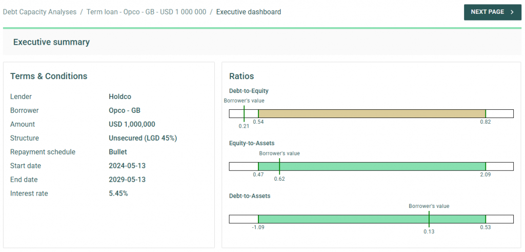
Today, we are thrilled to announce the launch of a new addition to our Transfer Pricing Suite: the Debt Capacity module. This innovative tool allows clients to build on their pricing analyses by quickly and accurately testing the debt capacity of borrower entities. Staying true to the essence of our Transfer Pricing Suite, the module is user-friendly yet delivers best-in-class support for tax compliance. 

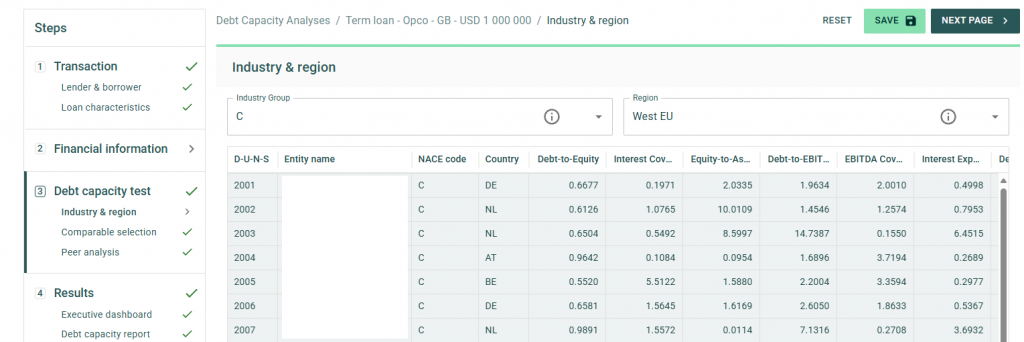
To streamline your in-house workflow, the standard package includes access to comparable data for a wide variety of borrowers. Within seconds, the application can automatically generate 40 comparable peers based on the borrower’s size, country, and industry through our connection with Dun & Bradstreet. Additionally, users can adjust and amend the list of comparable peers to ensure robust and tailored debt capacity tests for any scenario. 

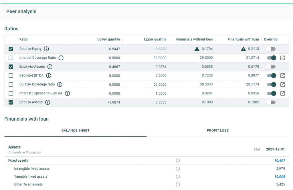
The debt capacity test leverages a flexible framework of financial ratios, which can be customized on a case-by-case basis. Our financial models dynamically adjust a borrower’s ratios to account for the impact of new loans on the balance sheet. With financial data for comparable entities readily available in the application, users receive feedback on debt capacity tests in under a minute. 

Upon completing the analysis, the application offers the option to generate a comprehensive report, available in Word or PDF formats. This detailed report outlines the methodology and underlying data used in the analysis, serving as an excellent complement to existing pricing reports and providing critical compliance support when it matters most. 

After releasing the initial version of the Debt Capacity module to clients, we will work on continuing to improve our applications. For example, by further supporting the debt capacity test through the inclusion of a dedicated cash flow forecast and an increase in comparable companies. If you’re interested in learning more, we invite you to contact our Transfer Pricing team to schedule a demo or trial the new module within your Zanders Inside environment. 

Zanders Transfer Pricing Solution   

 As tax authorities intensify their scrutiny, it is essential for companies to carefully adhere to the recommendations outlined above. Does this mean additional time and resources are required? Not necessarily. 

Technology provides an opportunity to minimize compliance risks while freeing up valuable time and resources. The Zanders Transfer Pricing Suite is an innovative, cloud-based solution designed to automate the transfer pricing compliance of financial transactions.  

With over seven years of experience and trusted by more than 80 multinational corporations, our platform is the market-leading solution for intra-group loans, guarantees, and cash pool transactions. 

Our clients trust us because we provide:  

• Transparent and high-quality embedded intercompany rating models.  

• A pricing model based on an automated search for comparable transactions.  

• Automatically generated, 40-page OECD-compliant Transfer Pricing reports.  

• Debt capacity analyses to support the quantum of debt.  

• Legal documentation aligned with the Transfer Pricing analysis.  

• Benchmark rates, sovereign spreads, and bond data included in the subscription.  

• Expert support from our Transfer Pricing specialists.  

• Quick and easy onboarding—completed within a day!  

Learn more, and discover the key compliance challenges for intra-group loan transfer pricing in 2025. 

Book a Demo

After a prolonged period of stable low (and at points even negative) interest rates, 2022 saw the return of rising rates, prompting Dutch digital bank, Knab, to appoint Zanders to reevaluate and reinforce the bank’s approach to risk.

The evolution of Knab

Founded in 2012 as the first fully digital bank in The Netherlands, Knab offers a suite of online banking products and services to support entrepreneurs both in their business and private needs.

“It's an underserved client group,” says Tom van Zalen, Knab’s Chief Risk Officer. “It's a nice niche as there is a strong need for a bank that really is there for these customers. We want to offer products and services that are really tailored to the specific needs of those entrepreneurs that often don’t fit the standard profile used in the market.”

Over time, the bank’s portfolio has evolved to offer a broad suite of online banking and financial services, including business accounts, mortgages, accounting tools, pensions and insurance. However, it was Knab’s mortgage portfolio that led them to be exposed to heightened interest rate risk. Mortgages with relatively long maturities command a large proportion of Knab’s balance sheet. When interest rates started to rise in 2022, increasing uncertainty in prepayments posed a significant risk to the bank. This emphasized the importance of upgrading their risk models to allow them to quantify the impact of changes in interest rates more accurately.

“With mortgages running for 20 plus years, that brings a certain interest rate risk,” says Tom. “That risk was quite well in control, until in 2022 interest rates started to change a lot. It became clear the risk models we were using needed to evolve and improve to align with the big changes we were observing in the interest rate environment—this was a very big thing we had to solve.”

In addition, in the background at around this time, major changes were happening in the ownership of the bank. This ultimately led to the sale of Knab (as part of Aegon NL) to a.s.r. in October 2022 and then to Bawag in February 2024. Although these transactions were not linked to the project we’re discussing here, they are relevant context as they represent the scale of change the bank was managing throughout this period, which added extra layers of complexity (and urgency) to the project.

A team effort

In 2022, Zanders was appointed by Knab to develop an Interest Rate Risk in the Banking Book (IRRBB) Roadmap that would enable them to navigate the changes in the interest rate environment, ensure regulatory compliance across their product portfolio and generally provide them with more control and clarity over their ALM position.  As a first stage of the project, Zanders worked closely with the Knab team to enhance the measurement of interest rate risk. The next stage of the project was then to develop and implement a new IRRBB strategy to manage and hedge interest rate risk more comprehensively and proactively by optimizing value risk, earnings risk and P&L. 

“The whole model landscape had to be redeveloped and that was a cumbersome and extensive process,” says Tom. “Redevelopment and validation took us seven to eight months. If you compare this to other banks, that sort of execution power is really impressive.”

The swiftness of the execution is the result of the high priority awarded to the project by the bank combined with the expertise of the Zanders team.

Zanders brings a very special combination of experts. Not only are they able to challenge the content and make sure we make the right choices, but they also bring in a market practice view. This combination was critical to the success of the execution of this project.

Tom van Zalen, Knab’s Chief Risk Officer.

Clarity and control

Armed with the new IRRBB infrastructure developed together with Zanders, the bank can now measure and monitor the interest rate risks in their product portfolio (and the impact on their balance sheet) more efficiently and with increased accuracy. This has empowered Knab with more control and clarity on their exposure to interest rate risk, enabling them to put the right measures in place to mitigate and manage risk effectively and compliantly.

“The model upgrade has helped us to reliably measure, monitor and quantify the risks in the balance sheet,” says Tom. “With these new models, the risk that we measure is now a real reflection of the actual risk. This has helped us also to rethink our approach on managing risk.”

The success of the project was qualified by an on-site inspection by the Dutch regulator, De Nederlandsche Bank (DNB), in April 2024. With Zanders supporting them, the Knab team successfully complied with regulatory requirements, and they were also complimented on the quality of their risk organization and management by the on-site inspection team.

Lasting impact

The success of the IRRBB Roadmap and the DNB inspection have really emphasized the extent of changes the project has driven across the bank’s processes. This was more than modeling risk, it was about embedding a more calculated and considered approach to risk management into the workings of the bank.

“It was not just a consultant flying in, doing their work and leaving again, it was really improving the bank,” says Tom. “If we look at where we are now, I really can say that we are in control of the risk, in the sense that we know where it is, we can measure it, we know what we need to do to manage it. And that is, a very nice position to be in.”

For more information on how Zanders can help you enhance your approach to interest rate risk, contact Erik Vijlbrief.

Over the past year, the interest rates on intercompany financial transactions have come under closer examination by tax authorities.  This intensified scrutiny stems from a mix of factors, including evolving regulations, more sophisticated audit procedures, the need from governments to boost revenue, and of course, high-interest-rate environment.  

As a result, these transactions are now being assessed with greater depth and rigor than ever before. Historically, tax authorities focused  on interest rate benchmarks as the primary point of analysis. However, their attention has now widened significantly to cover a range of interrelated considerations.  

Below is a brief overview of the key trends and areas attracting the most scrutiny in today’s landscape, highlighting what multinationals should pay attention to in 2025: 

Arm’s length T&Cs 

In the past years, tax authorities are closely examining the terms and conditions of intra-group debt, scrutinizing the pricing of loans and the effects of increased leverage.  

Accordingly, it is critical to ensure that the loan’s terms and conditions reflect the arm’s length standards and align with the actual economic substance of the transaction. This includes evaluating whether a hypothetical independent borrower, under similar conditions, could and would obtain a comparable loan.  

In addition to establishing an arm’s length interest rate and the appropriate amount of debt (further explained below), it is also necessary to assess whether the other terms and conditions are at arm’s length. This involves considering the main features of the loan—such as currency, maturity, repayment schedule, and callability—and evaluating their impact on the risk profile of both the borrower and the lender, as well as on the arm’s length interest rate. 

In this regard, tax authorities may challenge intra-group loans that do not include a maturity date, have an excessively long maturity (e.g., over 25 years), or lack a repayment schedule, since third-party loans would generally include these provisions.. They might also challenge situations where the actual conduct of the parties does not reflect the terms and conditions outlined in the loan agreement. For example, if the parties apply a different maturity or repayment schedule than the one initially agreed upon—without amending the legal documentation, which often happens in a dynamic intra-group financing environment—this could prompt further scrutiny from tax authorities. 

As a result, it is important for multinational enterprises to carefully consider these terms and conditions before issuing a loan, as they will have a direct impact on the interest rate applied in the transaction. Drafting a comprehensive loan agreement that clearly outlines these terms, aligns with the conditions applied in practice, and is supported by a robust Transfer Pricing analysis is recommended to mitigate the risk of challenges by tax authorities. 

Debt Capacity Analysis 

One of the most important terms and conditions that must meet arm’s length standards is the so-called quantum of debt (i.e. nominal amount of the loan extended). Tax authorities are increasingly scrutinizing whether the amount of intra-group debt is economically justified and supported by a clear business purpose. They also evaluate whether the debt aligns with arm’s length principles and serves a legitimate economic function consistent with the borrower’s overall business strategy. 

A debt capacity analysis is often conducted to determine whether the borrower has the financial capacity to repay the loan and whether an unrelated party would provide a similar amount of financing under comparable conditions. 

While many jurisdictions have long required this type of analysis in practice, Germany has taken a step further by formalizing this requirement under its 2024 Growth Opportunities Act. This was further clarified on December 12, 2024, when the German Federal Ministry of Finance issued administrative principles providing specific guidance on financing relationships under the new Transfer Pricing provisions. According to these principles, the debt capacity test hinges on two key criteria:  

(i) a credible expectation that the debtor can meet its obligations (e.g., interest payments and principal repayments),  

and (ii) a commitment to provide financing for a defined period.  

As a result, multinational enterprises are expected to robustly justify the level of debt assumed by their subsidiaries, particularly for entities operating in Germany. 

Credit Rating Analyses 

Tax authorities are increasing their focus on credit rating analyses. While simplified approaches, such as applying a uniform credit rating across all subsidiaries, were once more widely accepted, current practices favour a more detailed entity by entity evaluation. This involves first assigning a stand-alone credit rating to the individual borrower and then adjusting it to account for any implicit or explicit group support. 

In this context, Swiss tax authorities published last year a Q&A addressing various Transfer Pricing topics. In the section on financial transactions, they emphasized a clear preference for the bottom-up approach described above. This aligns closely with the OECD Transfer Pricing Guidelines and is consistent with the prevailing practices in most jurisdictions. 

In contrast, the administrative principles issued in Germany appear to take a different direction. According to the new rules, the arm’s-length nature of the interest rate for cross-border intercompany financing arrangements must generally be determined based on the group’s credit rating and external financing conditions. However, taxpayers are allowed to demonstrate that an alternative rating better aligns with the arm’s-length principle. 

This new approach diverges not only from the OECD guidelines but also from previous case law established by the German Federal Tax Court. As a result, several questions arise regarding how these rules will be applied in practice by German tax authorities. For instance, it remains unclear whether this approach will constitute a strict obligation or whether flexibility will be granted. Additionally, concerns exist about the burden of proof placed on taxpayers when opting for the bottom-up approach recommended by the OECD Transfer Pricing Guidelines. 

Cash Pool Synergy Distribution 

Tax authorities are increasingly aligning with Chapter X of the OECD Guidelines when evaluating cash pooling arrangements, with particular attention to the distribution of synergies among pool participants. 

According to the OECD Transfer Pricing Guidelines (Section C.2.3.2, paragraph 10.143), synergy benefits should generally be allocated to pool members by determining arm’s length interest rates that reflect each participant’s contributions and positions within the pool (e.g., debit or credit). 

Historically, the focus of tax authorities was primarily on the pricing methodologies— ensuring that both deposit and withdrawal margins were set at arm’s length. However, there is now a growing emphasis on how synergy benefits are distributed among participants. This is especially significant in jurisdictions where participants make substantial contributions to the pool balance. According to the OECD guidelines, these participants should benefit from the synergies generated by the pool through more favourable financing terms.  

To address these requirements and reduce the risk of disputes over cash pool structures, a three-step approach is recommended: 

1- Price the credit and debit positions of the participants. 

2- Calculate the synergy benefits generated within the structure. 

3- Allocate these benefits between the Cash Pool Leader and participants by adjusting the price applied to the participants.  

By following this approach, multinationals can ensure compliance with OECD guidelines and mitigate the likelihood of challenges from tax authorities. 

Zanders Transfer Pricing Solution  

As tax authorities intensify their scrutiny, it is essential for companies to carefully adhere to the recommendations outlined above.  

Does this mean additional time and resources are required? Not necessarily.  

Technology provides an opportunity to minimize compliance risks while freeing up valuable time and resources. The Zanders Transfer Pricing Suite is an innovative, cloud-based solution designed to automate the transfer pricing compliance of financial transactions.  

With over seven years of experience and trusted by more than 80 multinational corporations, our platform is the market-leading solution for intra-group loans, guarantees, and cash pool transactions. 

Our clients trust us because we provide: 

• Transparent and high-quality embedded intercompany rating models. 

• A pricing model based on an automated search for comparable transactions. 

• Automatically generated, 40-page OECD-compliant Transfer Pricing reports. 

• Debt capacity analyses to support the quantum of debt. 

• Legal documentation aligned with the Transfer Pricing analysis. 

• Benchmark rates, sovereign spreads, and bond data included in the subscription. 

• Expert support from our Transfer Pricing specialists. 

• Quick and easy onboarding—completed within a day! 

Book a Demo

Introduction: Faster, smarter, and future-proof 

In the fast-paced financial industry , speed and accuracy are paramount. Banks are tasked with the complex calculation of XVAs (‘X-Value Adjustments’) on a daily basis, which often involve computationally expensive Monte Carlo simulations. These calculations, while crucial, can become a bottleneck, slowing down decision-making processes and affecting efficiency. What if there is a faster and smarter way to handle these calculations? In this article, we explore a revolutionary approach that uses neural networks to drastically accelerate XVA calculations, promising significant speed-ups without sacrificing accuracy. 

The traditional approach: Monte Carlo simulations and their limitations 

Traditionally, banks have relied on Monte Carlo simulations to calculate XVAs. These simulations involve numerous complex scenarios, requiring substantial computational power and time. Imagine running simulations endlessly, with every tick of the clock translating to computing expenses. The problem? Time and resources. These calculations must be repeated daily, leading to significant delays and costs, potentially hindering your bank's responsiveness and decision-making agility. 

Despite bringing precision, this traditional method poses challenges. Given that the rates offered by banks do not fluctuate dramatically within days, repeating these extensive simulations seems redundant. This redundancy leads us to seek a solution that can deliver both speed and efficiency, paving the way for innovation. 

A new era: Leveraging Neural Networks for speed and efficiency 

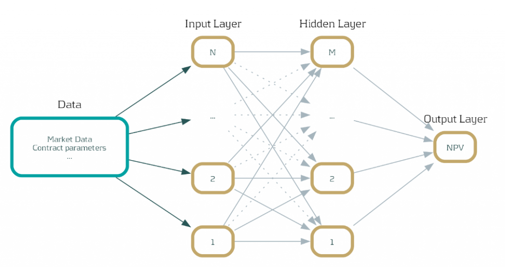
 Enter neural networks—an innovative technology that promises a solution to the Monte Carlo conundrum. By training these networks on Monte Carlo simulations conducted early in the week, such as on a Monday, the model can predict outcomes for the rest of the days. This approach sidesteps the need to perform cumbersome computations daily. 

Here’s how it works: The neural network learns from initial data, absorbing patterns and information that remain relatively constant through the week. This enables it to approximate net present value calculations with astonishing speed and accuracy. A practical example? Our integration of this technique into the Open-source Risk Engine resulted in a remarkable 600% increase in speed when assessing interest rate swap exposure in a stable market. 

Benefits of our solution: Integration and acceleration 

• Seamless Integration: Our solution can be seamlessly integrated with any existing systems, as long as they provide net present value outputs for some simulations. 

• Scalability with GPUs: Neural network calculations can harness the parallel processing power of GPUs, exponentially increasing inference speed. Imagine every inference equating to calculations for numerous trades simultaneously. 

• Feasibility and Reliability: With approximation of net present values being a commonly accepted practice in finance, this approach is both feasible and reliable for banks striving for rapid insights. 

Zanders Recommends: A strategic approach to implementation 

At Zanders, we believe in empowering banks with cutting-edge technology that aligns with their growth ambitions. Here is what we recommend: 

1- Assessment Phase: Evaluate the current computational model and identify areas that can benefit from the implementation of neural networks. 

2- Pilot Programs: Start with small-scale implementations to address specific bottlenecks and measure impact. 

3- Utilize GPUs: Leverage the parallelization capabilities of GPUs not just for neural networks but also for Monte Carlo simulations themselves, if needed. 

4- Continuous Improvement: Regularly update neural network models to ensure accuracy as market conditions evolve. 

Our extensive experience with high-performance computing, particularly the use of GPUs for parallelization, positions us as a trusted partner for banks navigating this transformation journey. 

Expertise spotlight: High-Performance Computing and AI solutions 

 In addition to revolutionizing XVA calculations, Zanders offers robust high-performance computing solutions that maximize the capabilities of GPUs across various applications, including Monte Carlo simulations. Our expertise also extends into AI technologies such as chatbots, where we implement and validate models, ensuring banks remain at the forefront of innovation. 

Conclusion: Embrace the future of banking technology 

 As the financial world evolves, so must the technologies that drive it. By leveraging neural networks, banks can achieve unprecedented speed and efficiency in XVA calculations, providing them with the agility needed to navigate today's dynamic markets. Now is the time to embrace a solution that is not only faster but smarter. At Zanders, we're ready to guide you through this transformation. Get in touch with Steven van Haren to learn how we can elevate your XVA calculations and ensure your bank stays competitive in an ever-changing financial landscape.

In the high-stakes world of Private Equity (PE), where exceptional returns are non-negotiable, value creation strategies have evolved far beyond financial engineering. Today, operational improvements, including in treasury and financial risk management, are required to yield high-quality returns. Among these, FX risk management often flies under the radar but holds significant untapped potential to protect and drive value for portfolio companies (PCs). In this article, we explore the importance of identifying and managing FX risks and suggest various quick wins to unlock value for portfolio companies.

The Untapped Potential of FX Risk Management in Value Creation 

PCs operating across multiple countries frequently lack a cohesive treasury and financial risk management approach. For example, bolt-on acquisitions often lead to fragmented teams, processes, systems and banking structures, while exposure to an increasing number of currencies creates financial risk that often remains invisible to central teams. This complexity is exacerbated by ad hoc and localized FX hedging practices, where PCs may not have access to competitive FX rates from their banking partners or access to a multi-bank FX dealing platform. 

For PE firms, FX risk often represents a hidden drain on EBITDA and cash flow. FX mismanagement can erode margins and impact portfolio company value. Hence the importance of uncovering financial and operational inefficiencies and building streamlined processes to manage FX exposures effectively. Proper FX risk management, which goes beyond hedging by means of financial instruments, not only mitigates financial risk but directly contributes to value creation by reducing cash flow volatility, reducing costs, increasing control, and increasing transparency. 

In this simplified example, a private equity-owned manufacturing firm, focused on expansion into emerging markets, was losing millions annually due to unmanaged foreign exchange (FX) exposures. The culprit? Decentralized treasury processes, idle bank balances in multiple currencies, and hidden FX risks within operational flows. The firm can address and manage these inefficiencies by using FX forward contracts to lock in exchange rates for future transactions and employing centralized treasury technology to monitor and control FX exposures across all operations. By addressing the inefficiencies, the firm reduced financial losses, stabilized its margins, and reinvested savings from FX gains into growth initiatives.

Quick Wins in FX Risk Management 

In your search of value creation, we suggest two potential quick wins to unlock PC value.  

Enhance Exposure Visibility 

Check whether your PCs operate with a clear understanding of their FX exposure landscape. Conducting a quick scan early in the investment lifecycle should identify, amongst others: 

• Where exposures are originated (e.g., revenues, costs, intercompany transactions) and if there are natural hedging possibilities. 

• Idle cash balances or loans in nonfunctional currencies, which create FX volatility. 

• The potential impact of these exposures on financial results through FX risk quantification. 

Private equity sponsors can facilitate the creation of a centralized treasury function that i) establishes a policy and process for FX risk management, ii) implements an FX dealing platform for efficient and competitive FX trading with banks, iii) monitors balances to reduce cash balances in non-functional currencies, and iv) implements netting arrangements to streamline intercompany payments and minimize cross-border transactions. 

Hidden FX Risk Discovery 

Business practices, such as allowing customers to pay in multiple currencies or a pricing agreement based on currency conversions, often lead to hidden FX risks and are a common pain point which is overlooked. For instance, a PC may receive customer payments in USD but agree to link the actual payable amount to the EUR/USD exchange rate, creating an implicit EUR exposure that impacts margins and cash flow.  

To address hidden FX risks, a private equity sponsor can help portfolio companies achieve a quick win by conducting a thorough analysis of their pricing models and operational agreements to identify implicit currency exposures, then implementing (soft) hedging techniques, such as adjusting pricing strategies to match revenue and cost currencies, renegotiating contracts with suppliers and customers to align payment terms, and utilizing natural hedging opportunities like balancing currency inflows and outflows, thereby minimizing net exposure before deciding to resort to financial instruments. 

In summary, as illustrated by the above quick wins, streamlining treasury processes can yield: 

• Hard dollar savings: Reduced FX costs by accessing competitive spreads. 

• Soft dollar savings: Enhanced decision-making through better visibility on exposures and reduced operational complexity. 

Consider this: A PE-owned retail chain expanded into international markets and faced profit erosion due to unmanaged FX risks and fragmented treasury processes. The sponsor conducted a quick scan to map exposures, uncovering mismatched revenue and expense currencies, a scattered landscape of bank accounts with idle balances, and operational inefficiencies. Hidden FX risks, such as supplier pricing tied to EUR/USD rates and uncoordinated customer payment options in multiple currencies, were also identified. Leveraging these insights, the sponsor centralized FX management by consolidating bank accounts, aligning supplier contracts with revenue streams to create natural hedges, and introducing competitive trading for FX transactions. They also established internal multilateral netting to streamline intercompany settlements, reducing FX costs by 20%.  

Measurable Results 

Integrating exposure identification and quantification, hidden risk discovery, and treasury process optimization into a single strategy enables PE firms to achieve more stable margins, cost savings, improved cash flow predictability and liberates capital for reinvestment. Furthermore, a proactive approach to FX risk management provides improved transparency for decision-making and LP reporting and strengthens financial resilience against market volatility. By embedding these robust treasury and financial risk management practices, PE sponsors can unlock hidden potential, ensuring their portfolio companies are not only protected but also positioned for sustainable growth and profitable exits.

Conclusion 

In the dynamic world of private equity, optimizing FX risk management for internationally operating PCs is a crucial strategy for safeguarding and enhancing portfolio value. Reflect on your current FX risk strategies and identify potential areas for improvement. Are there invisible exposures or inefficiencies limiting your portfolio’s growth? Take the initiative today - evaluate your FX risk management practices and make the necessary refinements to unlock substantial value for your portfolio companies. Embrace the opportunity to drive significant improvements in their financial resilience and overall performance. 

If you're interested in delving deeper into the benefits of strategic treasury management for private equity firms, please contact Job Wolters. 

The near-final PRA Rulebook PS9/24 published on 12 September 2024 includes substantial changes in credit risk regulation compared to the Consultation Paper CP16/22. While these amendments enhance clarity of Basel 3.1 implementation, institutions should conduct in-depth impact analysis to efficiently manage capital requirement. 

PRA has published draft proposal CP16/22 aligning closely with Basel 3.1 reforms. In response to industry feedback, the PRA has made material adjustments in PS9/24, which are aimed at better balancing alignment with international standards and maintaining the competitiveness of UK regulated institutions.  

Key takeaways 

1- Scope for a ‘Backstop’ revaluation every 5-years for valuation of real estate exposures 

2- SME and Infrastructure support factor is maintained, yet firm-specific adjustments will be introduced in pillar 2A. 

3- Despite industry concern on international competitiveness, the risk-sensitive approach for unrated corporate exposure is maintained. 

The implementation timeline is extended to 1 January 2026 with a 4-year transitional period, which is a one-year delay from the proposed implementation date of 1 January 2025 from CP16/22.

Real Estate Exposures  

According to the final regulations, the risk weights associated with regulatory real estate exposure will be calculated based on the type of property, the loan-to-value (LTV) ratio, and whether the repayments rely significantly on the cash flows produced by the property. In place of the potentially complex analysis proposed in CP16/22, the rules for determining whether a real estate exposure is materially dependent on cash flows have been significantly simplified and there is now a straightforward requirement for the classification of real estate exposures.  

One major change in the proposals relates to loans that are secured by commercial properties. The PRA has dropped the 100% risk weight floor for exposures backed by commercial real estate (CRE), provided that the repayment is not 'materially dependent on cash flows from the property' and that the exposure fits the 'regulatory real estate (RRE)' definition. Consequently, under the new rules, firms may, in some instances, benefit from low risk weights for commercial real estate, depending on the loan's loan-to-value (LTV) ratio and the type of counterparty involved. 

Additionally, the final rules regarding the revaluation of real estate have become more risk-sensitive. Although firms are still required to use the original valuation to calculate LTV, there is now a provision allowing for a ‘Backstop’ revaluation after five years. Going forward, the PRA has eliminated the need for firms to adjust valuations to reflect the 'prudent value' sustainable throughout the loan's duration. The requirements for downward revaluation have been simplified, mandating firms to reevaluate properties when they estimate a market value decline of over 10%. Furthermore, the PRA has specified that valuations can be conducted using a robust statistical model, such as an automated valuation model (AVM). 

SME support factor 

The PRA has maintained the draft proposal to remove the SME support factor under SA and IRB (Pillar 1), but has applied a firm-specific structural adjustment to Pillar 2A (the ‘SME lending adjustment’). The ‘SME lending adjustment’ aims to absorb the impact of removing the SME support factor in overall capital requirement.  

The PRA plans to communicate the adjusted Pillar 2 requirements to firms, ahead of the implementation date of the Basel 3.1 standards on 1 January 2026 (‘day 1’), so that firm-specific requirements will be updated at the same time as the Basel 3.1 standards are implemented. 

Infrastructure support factor 

The PRA has maintained the draft proposal to remove infrastructure support factor under SA and IRB approach, but has made two material changes which will diminish the impact on overall capital requirement.  

i. apply a firm-specific structural adjustment to Pillar 2A (the ‘SME lending adjustment’), which will minimize disruption in overall capital requirement. 

ii. introduce a new substantially stronger category in the slotting approach for IRB. PRA proposed lower risk-weight on the ‘substantially stronger’ IPRE exposures in CP16/22. The new definition of ‘substantially stronger’ is expected to include broader scope of IPRE exposures, thus lowering overall capital requirement. 

Unrated corporate exposures 

The PRA has maintained the draft proposal of introducing a two-way method on unrated corporate exposures: risk-sensitive and risk-neutral approach. Since the new approach does not apply in other jurisdictions, additional operational challenge is expected. Also, the 135% risk-weight on Non-IG(non-Investment Grade) unrated corporate exposure is higher than 100% in other jurisdictions, implying higher lending cost for UK regulated banks compared to its internationally regulated peers.

i. risk-sensitive approach : The PRA has proposed a risk-sensitive approach additional to the Basel III reforms. Exposures assessed by firms as IG would be risk-weighted at 65%, while exposures assessed by firms as Non-IG would be risk-weighted at 135%. This is a more risk-sensitive approach which aims to maintain an aggregate level of RWAs broadly consistent with the Basel III reforms.  

ii. risk-neutral approach: 100% risk weight is applied where the risk-sensitive approach is too costly or complex.  

In conclusion, the PRA's near-final Rulebook (PS9/24) reflects significant revisions to credit risk regulation that enhance clarity and alignment with Basel 3.1, while addressing industry feedback. The introduction of a five-year 'backstop' revaluation for real estate exposures, firm-specific adjustments for SMEs and infrastructure support factors, and the maintenance of a risk-sensitive approach for unrated corporate exposures underscore the PRA's commitment to balancing regulatory requirements with maintaining the competitiveness of UK institutions.  

The extended implementation timeline to 1 January 2026, along with the transitional period, allows firms adequate time for adjustment. Overall, these changes aim to foster a more robust and competitive banking environment, while also navigating the complexities introduced by differing international standards.  

How can Zanders help?  

We have extensive experience of implementation and validation of Pillar 1 & 2 models which allows us to effectively support our Clients managing the change process to full compliance with the latest regulations. 

From our experience, as the following are key areas on which our services can add most value: 

1- Carry out thorough self-assessment against new requirements including an impact analyses of new regulations on their capital requirements. 

2- Support model development activities to align models to new rules; we could be done either on an advisory basis or via direct supply of additional resources 

3- Support amendments to Pillar 2 models (which will have to reflect changes to Pillar 1 models) 

4- Support Internal Validation activities across Pillar 1 & 2 

5- Carry out quality assurance on final models & documentation before final submission to the PRA

6- Support adoption of solutions for prudential valuation of (real estate) collateral while integrating climate risk information. 

Please reach out to Paolo Vareschi or Suneet Dutta Roy to find out more about how we could support you on your journey to Basel 3.1 compliance. 

References

[1] Bank of England (2024), PS9/24 – Implementation of the Basel 3.1 standards near-final part 2 URL PS9/24 

[2] Bank of England (2022), CP16/22 – Implementation of the Basel 3.1 standards 
URL CP16/22