The Basel IV reforms, which are set to be implemented on 1 January 2025 via amendments to the EU Capital Requirement Regulation, have introduced changes to the Standardized Approach for credit risk (SA-CR). The Basel framework is implemented in the European Union mainly through the Capital Requirements Regulation (CRR3) and Capital Requirements Directive (CRD6). The CRR3 changes are designed to address shortcomings in the existing prudential standards, by among other items, introducing a framework with greater risk sensitivity and reducing the reliance on external ratings. Action by banks is required to remain compliant with the CRR. Overall, the share of RWEA derived through an external credit rating in the EU-27 remains limited, representing less than 10% of the total RWEA under the SA with the CRR.

Introduction

The Basel Committee on Banking Supervision (BCBS) identified the excessive dependence on external credit ratings as a flaw within the Standardised Approach (SA), observing that firms frequently used these ratings to compute Risk-Weighted Assets (RWAs) without adequately understanding the associated risks of their exposures. To address this issue, regulators have implemented changes aimed to reduce the mechanical reliance on external credit ratings and to encourage firms to use external credit ratings in a more informed manner. The objective is to diminish the chances of underestimating financial risks in order to further build a more resilient financial industry. Overall, the share of Risk Weighted Assets (RWA) derived through an external credit rating remains limited, and in Europe it represents less than 10% of the total RWA under the SA. 

The concept of due diligence is pivotal in the regulatory framework. It refers to the rigorous process financial institutions are expected to undertake to understand and assess the risks associated with their exposures fully. Regulators promote due diligence to ensure that banks do not solely rely on external assessments, such as credit ratings, but instead conduct their own comprehensive analysis.  

The due diligence is a process performed by banks with the aim of understanding the risk profile and characteristics of their counterparties at origination and thereafter on a regular basis (at least annually). This includes assessing the appropriateness of risk weights, especially when using external ratings. The level of due diligence should match the size and complexity of the bank's activities. Banks must evaluate the operating and financial performance of counterparties, using internal credit analysis or third-party analytics as necessary, and regularly access counterparty information. Climate-related financial risks should also be considered, and due diligence must be conducted both at the solo entity level and consolidated level. 

Banks must establish effective internal policies, processes, systems, and controls to ensure correct risk weight assignment to counterparties. They should be able to prove to supervisors that their due diligence is appropriate. Supervisors are responsible for reviewing these analyses and taking action if due diligence is not properly performed. 

Banks should have methodologies to assess credit risk for individual borrowers and at the portfolio level, considering both rated and unrated exposures. They must ensure that risk weights under the Standardised Approach reflect the inherent risk. If a bank identifies that an exposure, especially an unrated one, has higher inherent risk than implied by its assigned risk weight, it should factor this higher risk into its overall capital adequacy evaluation. 

Banks need to ensure they have an adequate understanding of their counterparties’ risk profiles and characteristics. The diligent monitoring of counterparties is applicable to all exposures under the SA. Banks would need to take reasonable and adequate steps to assess the operating and financial condition of each counterparty.

Rating System

The external credit assessment institutions (ECAIs) are credit rating agencies recognised by National supervisors. The External Credit ECAIs play a significant role in the SA through the mapping of each of their credit assessments to the corresponding risk weights. Supervisors will be responsible for assigning an eligible ECAI’s credit risk assessments to the risk weights available under the SA. The mapping of credit assessments should reflect the long-term default rate. 

Exposures to banks, exposures to securities firms and other financial institutions and exposures to corporates will be risk-weighted based on the following hierarchy External Credit Risk Assessment Approach (ECRA) and the Standardised Credit Risk Assessment Approach (SCRA). 

ECRA: Used in jurisdictions allowing external ratings. If an external rating is from an unrecognized or non-nominated ECAI, the exposure is considered unrated. Also, banks must perform due diligence to ensure ratings reflect counterparty creditworthiness and assign higher risk weights if due diligence reveals greater risk than the rating suggests. 

SCRA: Used where external ratings are not allowed. Applies to all bank exposures in these jurisdictions and unrated exposures in jurisdictions allowing external ratings. Banks classify exposures into three grades: 

• Grade A: Adequate capacity to meet obligations in a timely manner. 

• Grade B: Substantial credit risk, such as repayment capacities that are dependent on stable or favourable economic or business conditions. 

• Grade C: Higher credit risk, where the counterparty has material default risks and limited margins of safety 

The CRR Final Agreement includes a new article (Article 495e) that allows competent authorities to permit institutions to use an ECAI credit assessment assuming implicit government support until December 31, 2029, despite the provisions of Article 138, point (g). 

In cases where external credit ratings are used for risk-weighting purposes, due diligence should be used to assess whether the risk weight applied is appropriate and prudent.  

If the due diligence assessment suggests an exposure has higher risk characteristics than implied by the risk weight assigned to the relevant Credit Quality Step (CQS) of an exposure, the bank would assign the risk weight at least one higher than the CQS indicated by the counterparty’s external credit rating.

Criticisms to this approach are: 

1. Banks are mandated to use nominated ECAI ratings consistently for all exposures in an asset class, requiring banks to carry out a due diligence on each and every ECAI rating goes against the principle of consistent use of these ratings.  
2. When banks apply the output floor, ECAI ratings act as a backstop to internal ratings. In case the due diligence would imply the need to assign a high-risk weight, the output floor could no longer be used consistently across banks to compare capital requirements. 

Implementation Challenges

The regulation requires the bank to conduct due diligence to ensure a comprehensive understanding, both at origination and on a regular basis (at least annually), of the risk profile and characteristics of their counterparties. The challenges associated with implementing this regulation can be grouped into three primary categories: governance, business processes, and systems & data. 

Governance 

The existing governance framework must be enhanced to reflect the new responsibilities imposed by the regulation. This involves integrating the due diligence requirements into the overall governance structure, ensuring that accountability and oversight mechanisms are clearly defined. Additionally, it is crucial to establish clear lines of communication and decision-making processes to manage the new regulatory obligations effectively. 

Business Process 

A new business process for conducting due diligence must be designed and implemented, tailored to the size and complexity of the exposures. This process should address gaps in existing internal thresholds, controls, and policies. It is essential to establish comprehensive procedures that cover the identification, assessment, and monitoring of counterparties' risk profiles. This includes setting clear criteria for due diligence, defining roles and responsibilities, and ensuring that all relevant staff are adequately trained. 

Systems & Data 

The implementation of the regulation requires access to accurate and comprehensive data necessary for the rating system. Challenges may arise from missing or unavailable data, which are critical for assessing counterparties' risk profiles. Furthermore, reliance on manual solutions may not be feasible given the complexity and volume of data required. Therefore, it is imperative to develop robust data management systems that can capture, store, and analyse the necessary information efficiently. This may involve investing in new technology and infrastructure to automate data collection and analysis processes, ensuring data integrity and consistency. 

Overall, addressing these implementation challenges requires a coordinated effort across the organization, with a focus on enhancing governance frameworks, developing comprehensive business processes, and investing in advanced systems and data management solutions. 

How can Zanders help?  

As a trusted advisor, we built a track record of implementing CRR3 throughout a heterogeneous group of financial institutions. This provides us with an overview of how different entities in the industry deal with the different implementation challenges presented above.  

Zanders has been engaged to provide project management for these Basel IV implementation projects. By leveraging the expertise of Zanders' subject matter experts, we ensure an efficient and insightful gap analysis tailored to your bank's specific needs. Based on this analysis, combined with our extensive experience, we deliver customized strategic advice to our clients, impacting multiple departments within the bank. Furthermore, as an independent advisor, we always strive to challenge the status quo and align all stakeholders effectively. 

In-depth Portfolio Analysis: Our initial step involves conducting a thorough portfolio scan to identify exposures to both currently unrated institutions and those that rely solely on government ratings. This analysis will help in understanding the extent of the challenge and planning the necessary adjustments in your credit risk framework. 

Development of Tailored Models: Drawing from our extensive experience and industry benchmarks, Zanders will collaborate with your project team to devise a range of potential solutions. Each solution will be detailed with a clear overview of the required time, effort, potential impact on Risk-Weighted Assets (RWA), and the specific steps needed for implementation. Our approach will ensure that you have all the necessary information to make informed strategic decisions. 

Robust Solutions for Achieving Compliance: Our proprietary Credit Risk Suite cloud platform offers banks robust tools to independently assess and monitor the credit quality of corporate and financial exposures (externally rated or not) as well as determine the relevant ECRA and SCRA ratings. 

Strategic Decision-Making Support: Zanders will support your Management Team (MT) in the decision-making process by providing expert advice and impact analysis for each proposed solution. This support aims to equip your MT with the insights needed to choose the most appropriate strategy for your institution. 

Implementation Guidance: Once a decision has been made, Zanders will guide your institution through the specific actions required to implement the chosen solution effectively. Our team will provide ongoing support and ensure that the implementation is aligned with both regulatory requirements and your institution’s strategic objectives. 

Continuous Adaptation and Optimization: In response to the dynamic regulatory landscape and your bank's evolving needs, Zanders remains committed to advising and adjusting strategies as needed. Whether it's through developing an internal rating methodology, imposing new lending restrictions, or reconsidering business relations with unrated institutions, we ensure that your solutions are sustainable and compliant. 

Independent and Innovative Thinking: As an independent advisor, Zanders continuously challenges the status quo, pushing for innovative solutions that not only comply with regulatory demands but also enhance your competitive edge. Our independent stance ensures that our advice is unbiased and wholly in your best interest. 

By partnering with Zanders, you gain access to a team of dedicated professionals who are committed to ensuring your successful navigation through the regulatory complexities of Basel IV and CRR3. Our expertise and tailored approaches enable your institution to manage and mitigate risks efficiently while aligning with the strategic goals and operational realities of your bank. Reach out to Tim Neijs or Marco Zamboni for further comments or questions.

REFERENCE 

[1] BCBS, The Basel Framework, Basel https://www.bis.org/basel_framework 

[2] Regulation (EU) No 575/2013 

[3] Directive 2013/36/EU 

[4] EBA Roadmap on strengthening the prudential framework 

[5] EBA REPORT ON RELIANCE ON EXTERNAL CREDIT RATINGS 

The Covid-19 pandemic triggered unprecedented market volatility, causing widespread failures in banks' internal risk models. These backtesting failures threatened to increase capital requirements and restrict the use of advanced models. To avoid a potentially dangerous feedback loop from the lower liquidity, regulators responded by granting temporary exemptions for certain pandemic-related model exceptions. To act faster to future crises and reduce unreasonable increases to banks’ capital requirements, more recent regulation directly comments on when and how similar exemptions may be imposed.

Although FRTB regulation briefly comments on such situations of market stress, where exemptions may be imposed for backtesting and profit and loss attribution (PLA), it provides very little explanation of how banks can prove to the regulators that such a scenario has occurred. On 28^th June, the EBA published its final draft technical standards on extraordinary circumstances for continuing the use of internal models for market risk. These standards discuss the EBA’s take on these exemptions and provide some guidelines on which indicators can be used to identify periods of extreme market stresses.

Background and the BCBS

In the Basel III standards, the Basel Committee on Banking Supervision (BCBS) briefly comment on rare occasions of cross-border financial market stress or regime shifts (hereby called extreme stresses) where, due to exceptional circumstances, banks may fail backtesting and the PLA test. In addition to backtesting overages, banks often see an increasing mismatch between Front Office and Risk P&L during periods of extreme stresses, causing trading desks to fail PLA.

The BCBS comment that one potential supervisory response could be to allow the failing desks to continue using the internal models approach (IMA), however only if the banks models are updated to adequately handle the extreme stresses. The BCBS make it clear that the regulators will only consider the most extraordinary and systemic circumstances. The regulation does not, however, give any indication of what analysis banks can provide as evidence for the extreme stresses which are causing the backtesting or PLA failures.

The EBA’s standards

The EBA’s conditions for extraordinary circumstances, based on the BCBS regulation, provide some more guidance. Similar to the BCBS, the EBA’s main conditions are that a significant cross-border financial market stress has been observed or a major regime shift has taken place. They also agree that such scenarios would lead to poor outcomes of backtesting or PLA that do not relate to deficiencies in the internal model itself.

To assess whether the above conditions have been met, the EBA will consider the following criteria:

1. Analysis of volatility indices (such as the VIX and the VSTOXX), and indicators of realised volatilities, which are deemed to be appropriate to capture the extreme stresses,
2. Review of the above volatility analysis to check whether they are comparable to, or more extreme than, those observed during COVID-19 or the global financial crisis,
3. Assessment of the speed at which the extreme stresses took place,
4. Analysis of correlations and correlation indicators, which adequately capture the extreme stresses, and whether a significant and sudden change of them occurred,
5. Analysis of how statistical characteristics during the period of extreme stresses differ to those during the reference period used for the calibration of the VaR model.

The granularity of the criteria

The EBA make it clear that the standards do not provide an exhaustive list of suitable indicators to automatically trigger the recognition of the extreme stresses.  This is because they believe that cases of extreme stresses are very unique and would not be able to be universally captured using a small set of prescribed indicators.

They mention that defining a very specific set of indicators would potentially lead to banks developing automated or quasi-automated triggering mechanisms for the extreme stresses. When applied to many market scenarios, this may lead to a large number of unnecessary triggers due the specificity of the prescribed indicators. As such, the EBA advise that the analysis should take a more general approach, taking into consideration the uniqueness of each extreme stress scenario.

Responses to questions

The publication also summarises responses to the original Consultation Paper EBA/CP/2023/19. The responses discuss several different indicators or factors, on top of the suggested volatility indices, that could be used to identify the extreme stresses:

• The responses highlight the importance of correlation indicators. This is because stress periods are characterised by dislocations in the market, which can show increased correlations and heightened systemic risk.
• They also mention the use of liquidity indicators. This could include jumps of the risk-free rates (RFRs) or index swap (OIS) indicators. These liquidity indicators could be used to identify regime shifts by benchmarking against situations of significant cross-border market stress (for example, a liquidity crisis).
• Unusual deviations in the markets may also be strong indicators of the extreme stresses. For example, there could be a rapid widening of spreads between emerging and developed markets triggered by regional debt crisis. Unusual deviations between cash and derivatives markets or large difference between futures/forward and spot prices could also indicate extreme stresses.
• They suggest that restrictions on trading or delivery of financial instruments/commodities may be indicative of extreme stresses. For example, the restrictions faced by the Russian ruble due to the Russia-Ukraine war.
• Finally, the responses highlighted that an unusual amount of backtesting overages, for example more than 2 in a month, could also be a useful indicator.

Zanders recommends

It’s important that banks are prepared for potential extreme stress scenarios in the future. To achieve this, we recommend the following:

• Develop a holistic set of indicators and metrics that capture signs of potential extreme stresses,
• Use early warning signals to preempt potential upcoming periods of stress,
• Benchmark the indicators and metrics against what was observed during the great financial crisis and Covid-19,
• Create suitable reporting frameworks to ensure the knowledge gathered from the above points is shared with relevant teams, supporting early remediation of issues.

Conclusion

During extreme stresses such as Covid-19 and the global financial crisis, banks’ internal models can fail, not because of modelling issues but due to systemic market issues.  Under FRTB, the BCBS show that they recognise this and, in these rare situations, may provide exemptions. The EBA’s recently published technical standards provide better guidance on which indicators can be used to identify these periods of extreme stresses. Although they do not lay out a prescriptive and definitive set of indicators, the technical standards provide a starting point for banks to develop suitable monitoring frameworks.

For more information on this topic, contact Dilbagh Kalsi (Partner) or Hardial Kalsi (Manager).

Challenges with backtesting Expected Shortfall

Recent regulations are increasingly moving toward the use of Expected Shortfall (ES) as a measure to capture risk. Although ES fixes many issues with VaR, there are challenges when it comes to backtesting.

Although VaR has been widely-used for decades, its shortcomings have prompted the switch to ES. Firstly, as a percentile measure, VaR does not adequately capture tail risk. Unlike VaR, which gives the maximum expected portfolio loss in a given time period and at a specific confidence level, ES gives the average of all potential losses greater than VaR (see figure 1). Consequently, unlike Var, ES can capture a range of tail scenarios. Secondly, VaR is not sub-additive. ES, however, is sub-additive, which makes it better at accounting for diversification and performing attribution. As such, more recent regulation, such as FRTB, is replacing the use of VaR with ES as a risk measure.

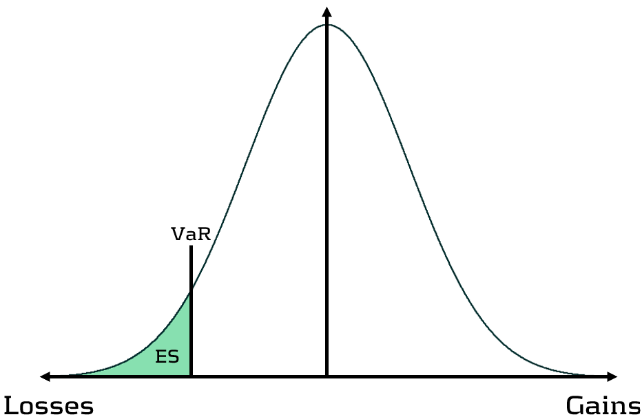
Figure 1: Comparison of VaR and ES

Elicitability is a necessary mathematical condition for backtestability. As ES is non-elicitable, unlike VaR, ES backtesting methods have been a topic of debate for over a decade. Backtesting and validating ES estimates is problematic – how can a daily ES estimate, which is a function of a probability distribution, be compared with a realised loss, which is a single loss from within that distribution? Many existing attempts at backtesting have relied on approximations of ES, which inevitably introduces error into the calculations.

The three main issues with ES backtesting can be summarised as follows:

1. Transparency
   • Without reliable techniques for backtesting ES, banks struggle to have transparency on the performance of their models. This is particularly problematic for regulatory compliance, such as FRTB.
2. Sensitivity
   • Existing VaR and ES backtesting techniques are not sensitive to the magnitude of the overages. Instead, these techniques, such as the Traffic Light Test (TLT), only consider the frequency of overages that occur.
3. Stability
   • As ES is conditional on VaR, any errors in VaR calculation lead to errors in ES. Many existing ES backtesting methodologies are highly sensitive to errors in the underlying VaR calculations.

Ridge Backtesting: A solution to ES backtesting

One often-cited solution to the ES backtesting problem is the ridge backtesting approach. This method allows non-elicitable functions, such as ES, to be backtested in a manner that is stable with regards to errors in the underlying VaR estimations. Unlike traditional VaR backtesting methods, it is also sensitive to the magnitude of the overages and not just their frequency.

The ridge backtesting test statistic is defined as:

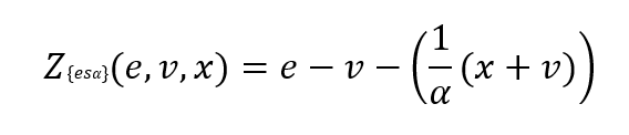
where 𝑣 is the VaR estimation, 𝑒 is the expected shortfall prediction, 𝑥 is the portfolio loss and 𝛼 is the confidence level for the VaR estimation.

The value of the ridge backtesting test statistic provides information on whether the model is over or underpredicting the ES. The technique also allows for two types of backtesting; absolute and relative. Absolute backtesting is denominated in monetary terms and describes the absolute error between predicted and realised ES. Relative backtesting is dimensionless and describes the relative error between predicted and realised ES. This can be particularly useful when comparing the ES of multiple portfolios. The ridge backtesting result can be mapped to the existing Basel TLT RAG zones, enabling efficient integration into existing risk frameworks.

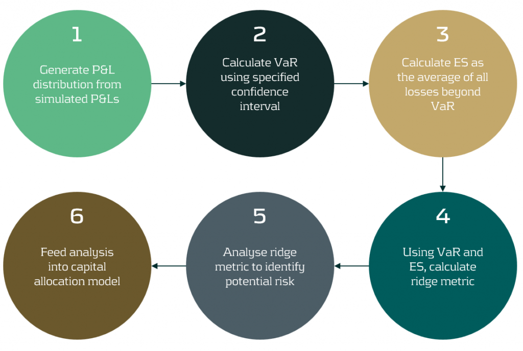
Figure 2: The ridge backtesting methodology

Sensitivity to Overage Magnitude

Unlike VaR backtesting, which does not distinguish between overages of different magnitudes, a major advantage of ES ridge backtesting is that it is sensitive to the size of each overage. This allows for better risk management as it identifies periods with large overages and also periods with high frequency of overages.

Below, in figure 3, we demonstrate the effectiveness of the ridge backtest by comparing it against a traditional VaR backtest. A scenario was constructed with P&Ls sampled from a Normal distribution, from which a 1-year 99% VaR and ES were computed. The sensitivity of ridge backtesting to overage magnitude is demonstrated by applying a range of scaling factors, increasing the size of overages by factors of 1, 2 and 3. The results show that unlike the traditional TLT, which is sensitive only to overage frequency, the ridge backtesting technique is effective at identifying both the frequency and magnitude of tail events. This enables risk managers to react more quickly to volatile markets, regime changes and mismodelling of their risk models.

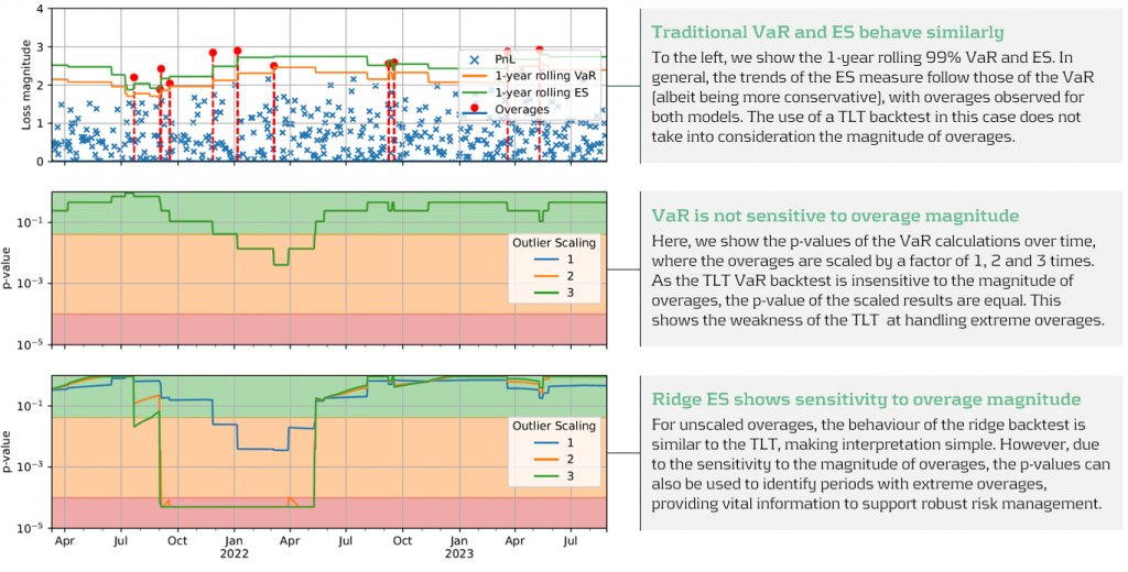
Figure 3: Demonstration of ridge backtesting’s sensitivity to overage magnitude.

The Benefits of Ridge Backtesting

Rapidly changing regulation and market regimes require banks enhance their risk management capabilities to be more reactive and robust. In addition to being a robust method for backtesting ES, ridge backtesting provides several other benefits over alternative backtesting techniques, providing banks with metrics that are sensitive and stable.

Despite the introduction of ES as a regulatory requirement for banks choosing the internal models approach (IMA), regulators currently do not require banks to backtest their ES models. This leaves a gap in banks’ risk management frameworks, highlighting the necessity for a reliable ES backtesting technique. Despite this, banks are being driven to implement ES backtesting methodologies to be compliant with future regulation and to strengthen their risk management frameworks to develop a comprehensive understanding of their risk.

Ridge backtesting gives banks transparency to the performance of their ES models and a greater reactivity to extreme events. It provides increased sensitivity over existing backtesting methodologies, providing information on both overage frequency and magnitude. The method also exhibits stability to any underlying VaR mismodelling.

In figure 4 below, we summarise the three major benefits of ridge backtesting.

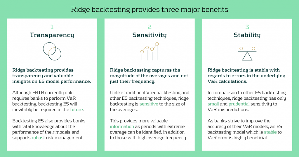
Figure 4: The three major benefits of ridge backtesting.

Conclusion

The lack of regulatory control and guidance on backtesting ES is an obvious concern for both regulators and banks. Failure to backtest their ES models means that banks are not able to accurately monitor the reliability of their ES estimates. Although the complexities of backtesting ES has been a topic of ongoing debate, we have shown in this article that ridge backtesting provides a robust and informative solution. As it is sensitive to the magnitude of overages, it provides a clear benefit in comparison to traditional VaR TLT backtests that are only sensitive to overage frequency. Although it is not a regulatory requirement, regulators are starting to discuss and recommend ES backtesting. For example, the PRA, EBA and FED have all recommended ES backtesting in some of their latest publications. However, despite the fact that regulation currently only requires banks to perform VaR backtesting, banks should strive to implement ES backtesting as it supports better risk management.

For more information on this topic, contact Dilbagh Kalsi (Partner) or Hardial Kalsi (Manager).

Across the whole of Europe, banks apply different techniques to model their IFRS9 Expected Credit Losses on a best estimate basis. The diverse spectrum of modelling techniques raises the question: what can we learn from each other, such that we all can improve our own IFRS 9 frameworks? For this purpose, Zanders hosted a webinar on the topic of IFRS 9 on the 29^th of May 2024. This webinar was in the form of a panel discussion which was led by Martijn de Groot and tried to discuss the differences and similarities by covering four different topics. Each topic was discussed by one  panelist, who were Pieter de Boer (ABN AMRO, Netherlands), Tobia Fasciati (UBS, Switzerland), Dimitar Kiryazov (Santander, UK), and Jakob Lavröd (Handelsbanken, Sweden).

The webinar showed that there are significant differences with regards to current IFRS 9 issues between European banks. An example of this is the lingering effect of the COVID-19 pandemic, which is more prominent in some countries than others. We also saw that each bank is working on developing adaptable and resilient models to handle extreme economic scenarios, but that it remains a work in progress. Furthermore, the panel agreed on the fact that SICR remains a difficult metric to model, and, therefore, no significant changes are to be expected on SICR models.

Covid-19 and data quality

The first topic covered the COVID-19 period and data quality. The poll question revealed widespread issues with managing shifts in their IFRS 9 model resulting from the COVID-19 developments. Pieter highlighted that many banks, especially in the Netherlands, have to deal with distorted data due to (strong) government support measures. He said this resulted in large shifts of macroeconomic variables, but no significant change in the observed default rate. This caused the historical data not to be representative for the current economic environment and thereby distorting the relationship between economic drivers and credit risk. One possible solution is to exclude the COVID-19 period, but this will result in the loss of data. However, including the COVID-19 period has a significant impact on the modelling relations. He also touched on the inclusion of dummy variables, but the exact manner on how to do so remains difficult.

Dimitar echoed these concerns, which are also present in the UK. He proposed using the COVID-19 period as an out-of-sample validation to assess model performance without government interventions. He also talked about the problems with the boundaries of IFRS 9 models. Namely, he questioned whether models remain reliable when data exceeds extreme values. Furthermore, he mentioned it also has implications for stress testing, as COVID-19 is a real life stress scenario, and we might need to think about other modelling techniques, such as regime-switching models.

Jakob found the dummy variable approach interesting and also suggested the Kalman filter or a dummy variable that can change over time. He pointed out that we need to determine whether the long term trend is disturbed or if we can converge back to this trend. He also mentioned the need for a common data pipeline, which can also be used for IRB models. Pieter and Tobia agreed, but stressed that this is difficult since IFRS 9 models include macroeconomic variables and are typically more complex than IRB.

Significant Increase in Credit Risk

The second topic covered the significant increase in credit risk (SICR). Jakob discussed the complexity of assessing SICR and the lack of comprehensive guidance. He stressed the importance of looking at the origination, which could give an indication on the additional risk that can be sustained before deeming a SICR.

Tobia pointed out that it is very difficult to calibrate, and almost impossible to backtest SICR. Dimitar also touched on the subject and mentioned that the SICR remains an accounting concept that has significant implications for the P&L. The UK has very little regulations on this subject, and only requires banks to have sufficient staging criteria. Because of these reasons, he mentioned that he does not see the industry converging anytime soon. He said it is going to take regulators to incentivize banks to do so. Dimitar, Jakob, and Tobia also touched upon collective SICR, but all agreed this is difficult to do in practice.

Post Model Adjustments

The third topic covered post model adjustments (PMAs). The results from the poll question implied that most banks still have PMAs in place for their IFRS 9 provisions. Dimitar responded that the level of PMAs has mostly reverted back to the long term equilibrium in the UK. He stated that regulators are forcing banks to reevaluate PMAs by requiring them to identify the root cause. Next to this, banks are also required to have a strategy in place when these PMAs are reevaluated or retired, and how they should be integrated in the model risk management cycle. Dimitar further argued that before COVID-19, PMAs were solely used to account for idiosyncratic risk, but they stayed around for longer than anticipated. They were also used as a countercyclicality, which is unexpected since IFRS 9 estimations are considered to be procyclical. In the UK, banks are now building PMA frameworks which most likely will evolve over the coming years.

Jakob stressed that we should work with PMAs on a parameter level rather than on ECL level to ensure more precise adjustments. He also mentioned that it is important to look at what comes before the modelling, so the weights of the scenarios. At Handelsbanken, they first look at smaller portfolios with smaller modelling efforts. For the larger portfolios, PMAs tend to play less of a role. Pieter added that PMAs can be used to account for emerging risks, such as climate and environmental risks, that are not yet present in the data. He also stressed that it is difficult to find a balance between auditors, who prefer best estimate provisions, and the regulator, who prefers higher provisions.

Linking IFRS 9 with Stress Testing Models

The final topic links IFRS 9 and stress testing. The poll revealed that most participants use the same models for both. Tobia discussed that at UBS the IFRS 9 model was incorporated into their stress testing framework early on. He pointed out the flexibility when integrating forecasts of ECL in stress testing. Furthermore, he stated that IFRS 9 models could cope with stress given that the main challenge lies in the scenario definition. This is in contrast with others that have been arguing that IFRS 9 models potentially do not work well under stress. Tobia also mentioned that IFRS 9 stress testing and traditional stress testing need to have aligned assumptions before integrating both models in each other.

Jakob agreed and talked about the perfect foresight assumption, which suggests that there is no need for additional scenarios and just puts a weight of 100% on the stressed scenario. He also added that IFRS 9 requires a non-zero ECL, but a highly collateralized portfolio could result in zero ECL. Stress testing can help to obtain a loss somewhere in the portfolio, and gives valuable insights on identifying when you would take a loss. 

Pieter pointed out that IFRS 9 models differ in the number of macroeconomic variables typically used. When you are stress testing variables that are not present in your IFRS 9 model, this could become very complicated. He stressed that the purpose of both models is different, and therefore integrating both can be challenging. Dimitar said that the range of macroeconomic scenarios considered for IFRS 9 is not so far off from regulatory mandated stress scenarios in terms of severity. However, he agreed with Pieter that there are different types of recessions that you can choose to simulate through your IFRS 9 scenarios versus what a regulator has identified as systemic risk for an industry. He said you need to consider whether you are comfortable relying on your impairment models for that specific scenario.

This topic concluded the webinar on differences and similarities across European countries regarding IFRS 9. We would like to thank the panelists for the interesting discussion and insights, and the more than 100 participants for joining this webinar.

Interested to learn more? Contact Kasper Wijshoff, Michiel Harmsen or Polly Wong for questions on IFRS 9.

In January 2022, the OECD incorporated Chapter X to the latest edition of their Transfer Pricing Guidelines, a pivotal step in regulating financial transactions globally. This addition aimed to set a global standard for transfer pricing of intercompany financial transactions, an area long scrutinized for its potential for profit shifting and tax avoidance. In the years since, we have seen various jurisdictions explicitly incorporating these principles and providing further guidance in this area. Notably, in the last year, we saw new guidance in South Africa, Germany, and the United Arab Emirates (UAE), while the Swiss and American tax authorities offered more explanations on this topic. In this article we will take you through the most important updates for the coming years.

Finding the right comparable

The arm's length principle established in the OECD Transfer Pricing Guidelines stipulates that the price applied in any intra-group transaction should be as if the parties were independent.¹ This principle applies equally to financial transactions: every intra-group loan, guarantee, and cash pool should be priced in a manner that would be reasonable for independent market participants. Chapter X of the OECD Guidelines provided for the first time a detailed guidance on applying the arm's length principle to financial transactions. Since its publication, achieving arm's length pricing for financial transactions has become a significant regulatory challenge for many multinational corporations. At the same time the increased interest rates have encouraged tax authorities to pay increased attention to the topic – strengthened with the guidelines from Chapter X. 

To determine the arm’s length price of an intra-group financial transaction, the most common methodology is to search for comparable market transactions that share the characteristics of the internal transaction under analysis. For example, in terms of credit risk, maturity, currency or the presence of embedded options. In the case of financial transactions, these comparable market transactions are often loans, traded bonds, or publicly available deposit facilities. Using these comparable observations, an estimate is made on the appropriate price of a transaction as a compensation for the risk taken by either party in a transaction. The risk-adjusted rate of return incorporates the impact of the borrower’s credit rating, any security present, the time to maturity of the transaction, and any other features that are deemed relevant. This methodology has been explicitly incorporated in many publications including in the guidance from the South African Revenue Service (SARS)² and the Administrative Principles 2023 from the German Federal Ministry of Finance.³

The recently published Corporate Tax Guide of the UAE also implements OECD Chapter X, but does not explicitly mention a preference for market instruments. Instead, the tax guide prefers the use of “comparable debt instruments” without offering examples of appropriate instruments. This nuance requires taxpayers to describe and defend their selection of instruments for each type of transaction. Although the regulation allows for comparability adjustments for differences in terms and conditions, the added complexity poses an additional challenge for many taxpayers. 

A special case of financial transaction for transfer pricing are cash pooling structures. Due to the multilateral nature of cash pools, a single benchmark study might be insufficient. OECD Chapter X introduced the principle of synergy allocation in a cash pool, where the benefits of the pool are shared between its leader and the participants of the pool based on the functions performed and risks assumed. This synergy allocation approach is also found in the recent guidance of SARS, but not in the German Administrative Principles. Instead, the German authorities suggest a cost-plus compensation for a leader of a cash pool with limited risks and functionality. Surprisingly, approaches for complex cash pooling structures such as an in-house bank are not described by the new German Administrative Principles.  

To find out more about the search for the best comparable, have a look at our white paper. You can download a free copy here.

Moving towards new credit rating analyses

Before pricing an intra-group financial transaction, it is paramount to determine the credit risks attached to the transaction under analysis. This can be a challenging exercise, as the borrowing entity is rarely a stand-alone entity which has public debt outstanding or a public credit rating. As a result, corporates typically rely on a top-down or bottom-up rating analysis to estimate the appropriate credit risk in a transaction. In a top-down analysis, the credit rating is largely based on the strength of the group: the subsidiary credit rating is derived by downgrading the group rating by one or two notches. An alternative approach is the bottom-up analysis, where the stand-alone creditworthiness of the borrower is first assessed through its financial statements. Afterwards, the stand-alone credit rating is adjusted with the group’s credit rating based on the level of support that the subsidiary can derive from the group. 

The group support assessment is an important consideration in the credit rating assessment of subsidiaries. Although explicit guarantees or formal support between an entity and the group are often absent, it should still be assessed whether the entity benefits from association with the group: implicit group support. Authorities in the United States, Switzerland, and Germany have provided more insight into their views on the role of the implicit group support, all of them recognizing it as a significant factor that needs to be considered in the credit rating analysis. For instance, the American Internal Revenue Service emphasized the impact of passive association of an entity with the group in the memorandum issued in December 2023.⁴

The Swiss tax authorities have also stressed the importance of implicit support for rating analyses in the Q&A released in February 2024.⁵ In this guidance, the authorities did not only emphasize the importance of factoring the implicit group support, but also expressed a preference for the bottom-up approach. This contrasts with the top-down approach followed by many multinationals in the past, which are now encouraged to adopt a more comprehensive method aligned with the bottom-up approach.

Interested in learning more about credit ratings? Our latest white paper has got you covered!
Grab a free copy here.

Standardization for success

Although the standards set by the OECD have been explicitly adopted by numerous jurisdictions, the additional guidance further develops the requirements in complex transfer pricing areas. Navigating such a complex and demanding environment under increasing interest rates is a challenge for many multinational corporations. Perhaps the best advice is found in the German publication: in its Administrative Principles, it is stressed that the transfer price determination should occur before completion of the transaction and the guidelines prefer a standardized methodology. To get a head start, it is important to put in place an easy to execute process for intra-group financial transactions with comprehensive transfer pricing documentation.  

Despite the complexity of the topic involved, such a standardized method will always be easier to defend. One thing is for certain: the details of transfer pricing studies for financial transactions, such as the analysis of ratings and the debt market, will continue to be a part of every transfer pricing and tax manager agenda for 2024.

For more information on Mastering Financial Transaction Transfer Pricing, download our white paper.

In countries worldwide, associations of credit information providers play a crucial role in registering consumer-related credits. They are mandated by regulation, operate under local law and their primary aim is consumer protection. The Dutch Central Credit Registration Agency, Stichting Bureau Krediet Registratie (BKR), has reviewed the validity of the credit registration period, especially with regards to the recurrence of payment problems after the completion of debt restructuring and counseling. Since 2017, Zanders and BKR are cooperating in quantitative research and modeling projects and they joined forces for this specific research.

In the current Dutch public discourse, diverse opinions regarding the retention period after finishing debt settlements exist and discussions have started to reduce the duration of such registrations. In December 2022, the four biggest municipalities in the Netherlands announced their independent initiative to prematurely remove registrations of debt restructuring and/or counseling from BKR six months after finalization. Secondly, on 21 June 2023, the Minister of Finance of the Netherlands published a proposal for a Credit Registration System Act for consultation, including a proposition to shorten the retention period in the credit register from five to three years. This proposition will also apply to credit registrations that have undergone a debt rescheduling.

The Dutch Central Credit Registration Agency, Stichting Bureau Krediet Registratie (BKR) receives and manages credit registrations and payment arrears of individuals in the Netherlands. By law, a lender in the Netherlands must verify whether an applicant already has an existing loan when applying for a new one. Additionally, lenders are obligated to report every loan granted to a credit registration agency, necessitating a connection with BKR. Besides managing credit data, BKR is dedicated to gathering information to prevent problematic debt situations, prevent fraud, and minimize financial risks associated with credit provision. As a non-profit foundation, BKR operates with a focus on keeping the Dutch credit market transparent and available for all.

BKR recognizes that the matter concerning the retention period of registrations for debt restructuring and counseling is fundamentally of societal nature. Many stakeholders are concerned with the current discussions, including municipalities, lenders and policymakers. To foster public debate on this matter, BKR is committed to conducting an objective investigation using credit registration data and literature sources and has thus engaged Zanders for this purpose. By combining expertise in financial credit risk with data analysis, Zanders offers unbiased insights into this issue. These data-driven insights are valuable for BKR, lawmakers, lenders, and municipalities concerning retention periods, payment issues, and debt settlements.

Problem Statement

The Dutch Central Credit Registration Agency, Stichting Bureau Krediet Registratie (BKR) receives and manages credit registrations and payment arrears of individuals in the Netherlands. By law, a lender in the Netherlands must verify whether an applicant already has an existing loan when applying for a new one. Additionally, lenders are obligated to report every loan granted to a credit registration agency, necessitating a connection with BKR. Besides managing credit data, BKR is dedicated to gathering information to prevent problematic debt situations, prevent fraud, and minimize financial risks associated with credit provision. As a non-profit foundation, BKR operates with a focus on keeping the Dutch credit market transparent and available for all.

The research aims to gain a deeper understanding of the recurrence of payment issues following the completion of restructuring credits (recidivism). The information gathered will aid in shaping thoughts about an appropriate retention period for the registration of finished debt settlements. The research includes both qualitative and quantitative investigations. The qualitative aspect involves a literature study, leading to an overview of benchmarking, key findings and conclusions from prior studies on this subject. The quantitative research comprises data analyses on information from BKR's credit register.

External International Qualitative Research

The literature review encompassed several Dutch and international sources that discuss debt settlements, credit registrations, and recidivism. There is limited research published on recidivism, but there are some actual cases where retention period are materially shortened or credit information is deleted to increase access to financial markets for borrowers. Removing information increases information asymmetry, meaning that borrower and lender do not have the same insights limiting lenders to make well-informed decisions during the credit application process. The cases in which the retention period was shortened or negative credit registrations were removed demonstrate significant consequences for both consumers and lenders. Such actions led to higher default rates, reduced credit availability, and increased credit costs, also for private individuals without any prior payment issues.

In the literature it is described that historical credit information serves as predictive variable for payment issues, emphasizing the added value of credit registrations in credit reports, showing that this mitigates the risk of overindebtedness for both borrowers and lenders.

Quantitative Research with Challenges and Solutions

BKR maintains a large data set with information regarding credits, payment issues, and debt settlements. For this research, data from over 2.5 million individuals spanning over 14 years were analyzed. Transforming this vast amount of data into a usable format to understand the payment and credit behavior of individuals posed a challenge.

The historical credit registration data has been assessed to (i) gain deeper insights into the relationship between the length of retention periods after debt restructuring and counseling and new payment issues and (ii) determine whether a shorter retention period after the resolution of payment issues negatively impacts the prevention of new payment issues, thus contributing to debt prevention to a lesser extent.

The premature removal of individuals from the system of BKR presented an additional challenge. Once a person’s information is removed from the system, their future payment behavior can no longer be studied. Additionally, the group subject to premature removal (e.g. six months to a year) after a debt settlement registration constitutes only a small portion of the population, making research on this group challenging. To overcome these challenges, the methodology was adapted to assess the outflow of individuals over time, such that conclusions about this group could still be made.

Conclusion

The research provided BKR with several interesting conclusions. The data supported the literature that there is difference in risk for payment issues between lenders with and without debt settlement history. Literature shows that reducing the retention period increases the access to the financial markets for those finishing a debt restructuring or counseling. It also increases the risk in the financial system due to the increased information asymmetry between lender and borrower, with several real-life occasions with

increased costs and reduced access to lending for all private individuals. The main observation of the quantitative research is that individuals who have completed a debt rescheduling or debt counseling face a higher risk of relapsing into payment issues compared to those without debt restructuring or counseling history. An outline of the research report is available on the website of BKR.

The collaboration between BKR and Zanders has fostered a synergy between BKR's knowledge, data, and commitment to research and Zanders' business experience and quantitative data analytical skills. The research provides an objective view and quantitative and qualitative insights to come to a well informed decision about the optimal registration period for the credit register. It is up to the stakeholders to discuss and decide on the way forward.

Under FRTB regulation, PLA requires banks to assess the similarity between Front Office (FO) and Risk P&L (HPL and RTPL) on a quarterly basis. Desks which do not pass PLA incur capital surcharges or may, in more severe cases, be required to use the more conservative FRTB standardised approach (SA).​

What is the purpose of PLA?​

PLA ensures that the FO and Risk P&Ls are sufficiently aligned with one another at the desk level.​ The FO HPL is compared with the Risk RTPL using two statistical tests.​ The tests measure the materiality of any simplifications in a bank’s Risk model compared with the FO systems.​ In order to use the Internal Models Approach (IMA), FRTB requires each trading desk to pass the PLA statistical tests.​ Although the implementation of PLA begins on the date that the IMA capital requirement becomes effective, banks must provide a one-year PLA test report to confirm the quality of the model.

Which statistical measures are used?​

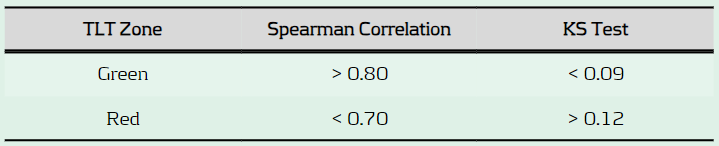
PLA is performed using the Spearman Correlation and the Kolmogorov-Smirnov (KS) test using the most recent 250 days of historical RTPL and HPL.​ Depending on the results, each desk is assigned a traffic light test (TLT) zone (see below), where amber desks are those which are allocated to neither red or green.​

What are the consequences of failing PLA?

Capital increase: Desks in the red zone are not permitted to use the IMA and must instead use the more conservative SA, which has higher capital requirements. ​Amber desks can use the IMA but must pay a capital surcharge until the issues are remediated.

Difficulty with returning to IMA: Desks which are in the amber or red zone must satisfy statistical green zone requirements and 12-month backtesting requirements before they can be eligible to use the IMA again.​

What are some of the key reasons for PLA failure?

Data issues: Data proxies are often used within Risk if there is a lack of data available for FO risk factors. Poor or outdated proxies can decrease the accuracy of RTPL produced by the Risk model.​ The source, timing and granularity also often differs between FO and Risk data.

Missing risk factors: Missing risk factors in the Risk model are a common cause of PLA failures. Inaccurate RTPL values caused by missing risk factors can cause discrepancies between FO and Risk P&Ls and lead to PLA failures.

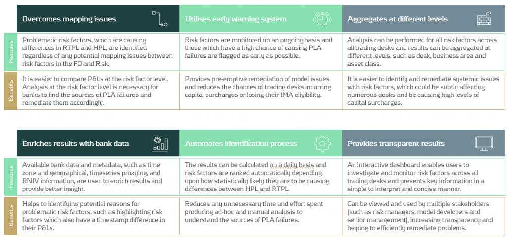
Roadblocks to finding the sources of PLA failures

FO and Risk mapping: Many banks face difficulties due to a lack of accurate mapping between risk factors in FO and those in Risk. ​For example, multiple risk factors in the FO systems may map to a single risk factor in the Risk model. More simply, different naming conventions can also cause issues.​ The poor mapping can make it difficult to develop an efficient and rapid process to identify the sources of P&L differences.

Lack of existing processes: PLA is a new requirement which means there is a lack of existing infrastructure to identify causes of P&L failures. ​Although they may be monitored at the desk level, P&L differences are not commonly monitored at the risk factor level on an ongoing basis.​ A lack of ongoing monitoring of risk factors makes it difficult to pre-empt issues which may cause PLA failures and increase capital requirements.

Our approach: Identifying risk factors that are causing PLA failures

Zanders’ approach overcomes the above issues by producing analytics despite any underlying mapping issues between FO and Risk P&L data. ​Using our algorithm, risk factors are ranked depending upon how statistically likely they are to be causing differences between HPL and RTPL.​ Our metric, known as risk factor ‘alpha’, can be tracked on an ongoing basis, helping banks to remediate underlying issues with risk factors before potential PLA failures.

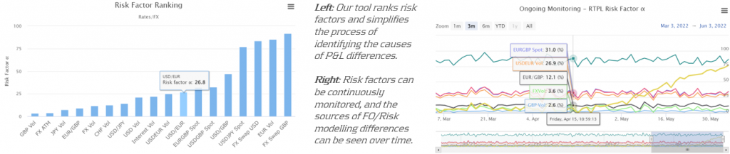
Zanders’ P&L attribution solution has been implemented at a Tier-1 bank, providing the necessary infrastructure to identify problematic risk factors and improve PLA desk statuses. The solution provided multiple benefits to increase efficiency and transparency of workstreams at the bank.

Conclusion

As it is a new regulatory requirement, passing the PLA test has been a key concern for many banks. Although the test itself is not considerably difficult to implement, identifying why a desk may be failing can be complicated. In this article, we present a PLA tool which has already been successfully implemented at one of our large clients. By helping banks to identify the underlying risk factors which are causing desks to fail, remediation becomes much more efficient. Efficient remediation of desks which are failing PLA, in turn, reduces the amount of capital charges which banks may incur.

Challenges with VaR models in a turbulent market​

With recent periods of market stress, including COVID-19 and the Russia-Ukraine conflict, banks are finding their VaR models under strain. A failure to adhere to VaR backtesting requirements can lead to pressure on balance sheets through higher capital requirements and interventions from the regulator.

VaR backtesting

VaR is integral to the capital requirements calculation and in ensuring a sufficient capital buffer to cover losses from adverse market conditions.​ The accuracy of VaR models is therefore tested stringently with VaR backtesting, comparing the model VaR to the observed hypothetical P&Ls. ​A VaR model with poor backtesting performance is penalised with the application of a capital multiplier, ensuring a conservative capital charge.​ The capital multiplier increases with the number of exceptions during the preceding 250 business days, as described in Table 1 below.​

Table 1: Capital multipliers based on the number of backtesting exceptions.

The capital multiplier is applied to both the VaR and stressed VaR, as shown in equation 1 below, which can result in a significant impact on the market risk capital requirement when failures in VaR backtesting occur.​

Pro-cyclicality of the backtesting framework​

A known issue of VaR backtesting is pro-cyclicality in market risk. ​This problem was underscored at the beginning of the COVID-19 outbreak when multiple banks registered several VaR backtesting exceptions. ​This had a double impact on market risk capital requirements, with higher capital multipliers and an increase in VaR from higher market volatility.​ Consequently, regulators intervened to remove additional pressure on banks’ capital positions that would only exacerbate market volatility. The Federal Reserve excluded all backtesting exceptions between 6th – 27th March 2020, while the PRA allowed a proportional reduction in risks-not-in-VaR (RNIV) capital charge to offset the VaR increase.​ More recent market volatility however has not been excluded, putting pressure on banks’ VaR models during backtesting.​

Historical simulation VaR model challenges​

Banks typically use a historical simulation approach (HS VaR) for modelling VaR, due to its computational simplicity, non-normality assumption of returns and enhanced interpretability. ​Despite these advantages, the HS VaR model can be slow to react to changing markets conditions and can be limited by the scenario breadth. ​This means that the HS VaR model can fail to adequately cover risk from black swan events or rapid shifts in market regimes.​ These issues were highlighted by recent market events, including COVID-19, the Russia-Ukraine conflict, and the global surge in inflation in 2022.​ Due to this, many banks are looking at enriching their VaR models to better model dramatic changes in the market.

Enriching HS VaR models​

Alternative VaR modelling approaches can be used to enrich HS VaR models, improving their response to changes in market volatility. Volatility scaling is a computationally efficient methodology which can resolve many of the shortcomings of HS VaR model, reducing backtesting failures.​

Enhancing HS VaR with volatility scaling​

The Volatility Scaling methodology is an extension of the HS VaR model that addresses the issue of inertia to market moves.​ Volatility scaling adjusts the returns for each time t by the volatility ratio σT/σt, where σt is the return volatility at time t and σT is the return volatility at the VaR calculation date.​ Volatility is calculated using a 30-day window, which more rapidly reacts to market moves than a typical 1Y VaR window, as illustrated in Figure 1.​ As the cost of underestimation is higher than overestimating VaR, a lower bound to the volatility ratio of 1 is applied.​ Volatility scaling is simple to implement and can enrich existing models with minimal additional computational overhead.​

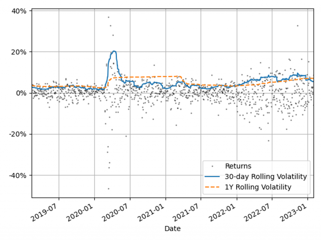
Figure 1: The 30-day and 1Y rolling volatilities of the 1-day scaled diversified portfolio returns. This illustrates recent market stresses, with short regions of extreme volatility (COVID-19) and longer systemic trends (Russia-Ukraine conflict and inflation). 

Comparison with alternative VaR models​

To benchmark the Volatility Scaling approach, we compare the VaR performance with the HS and the GARCH(1,1) parametric VaR models.​ The GARCH(1,1) model is configured for daily data and parameter calibration to increase sensitivity to market volatility.​ All models use the 99th percentile 1-day VaR scaled by a square root of 10. ​The effective calibration time horizon is one year, approximated by a VaR window of 260 business days.​ A one-week lag is included to account for operational issues that banks may have to load the most up-to-date market data into their risk models.​

VaR benchmarking portfolios​

To benchmark the VaR Models, their performance is evaluated on several portfolios that are sensitive to the equity, rates and credit asset classes. ​These portfolios include sensitivities to: S&P 500 (Equity), US Treasury Bonds (Treasury), USD Investment Grade Corporate Bonds (IG Bonds) and a diversified portfolio of all three asset classes (Diversified).​ This provides a measure of the VaR model performance for both diversified and a range of concentrated portfolios.​ The performance of the VaR models is measured on these portfolios in both periods of stability and periods of extreme market volatility. ​This test period includes COVID-19, the Russia-Ukraine conflict and the recent high inflationary period.​

VaR model benchmarking

The performance of the models is evaluated with VaR backtesting. The results show that the volatility scaling provides significantly improved performance over both the HS and GARCH VaR models, providing a faster response to markets moves and a lower instance of VaR exceptions.​

Model benchmarking with VaR backtesting​

A key metric for measuring the performance of VaR models is a comparison of the frequency of VaR exceptions with the limits set by the Basel Committee’s Traffic Light Test (TLT). ​Excessive exceptions will incur an increased capital multiplier for an Amber result (5 – 9 exceptions) and an intervention from the regulator in the case of a Red result (ten or more exceptions).​ Exceptions often indicate a slow reaction to market moves or a lack of accuracy in modelling risk.​

VaR measure coverage​

The coverage and adaptability of the VaR models can be observed from the comparison of the realised returns and VaR time series shown in Figure 2.​ This shows that although the GARCH model is faster to react to market changes than HS VaR, it underestimates the tail risk in stable markets, resulting in a higher instance of exceptions.​ Volatility scaling retains the conservatism of the HS VaR model whilst improving its reactivity to turbulent market conditions. This results in a significant reduction in exceptions throughout 2022.​

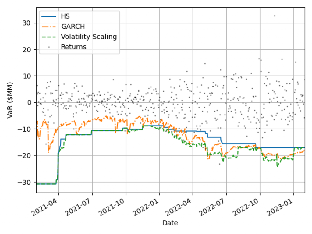
Figure 2: Comparison of realised returns with the model VaR measures for a diversified portfolio.

VaR backtesting results​

The VaR model performance is illustrated by the percentage of backtest days with Red, Amber and Green TLT results in Figure 3.​ Over this period HS VaR shows a reasonable coverage of the hypothetical P&Ls, however there are instances of Red results due to the failure to adapt to changes in market conditions.​ The GARCH model shows a significant reduction in performance, with 32% of test dates falling in the Red zone as a consequence of VaR underestimation in calm markets.​ The adaptability of volatility scaling ensures it can adequately cover the tail risk, increasing the percentage of Green TLT results and completely eliminating Red results.​ In this benchmarking scenario, only volatility scaling would pass regulatory scrutiny, with HS VaR and GARCH being classified as flawed models, requiring remediation plans.

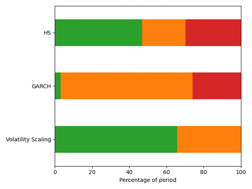
Figure 3: Percentage of days with a Red, Amber and Green Traffic Light Test result for a diversified portfolio over the window 29/01/21 - 31/01/23.

VaR model capital requirements​

Capital requirements are an important determinant in banks’ ability to act as market intermediaries. The volatility scaling method can be used to increase the HS capital deployment efficiency without compromising VaR backtesting results.​

Capital requirements minimisation​

A robust VaR model produces risk measures that ensure an ample capital buffer to absorb portfolio losses. When selecting between robust VaR models, the preferred approach generates a smaller capital charge throughout the market cycle. Figure 4 shows capital requirements for the VaR models for a diversified portfolio calculated using Equation 1, with 𝐴𝑑𝑑𝑜𝑛𝑠 set to zero. Volatility scaling outperforms both models during extreme market volatility (the Russia-Ukraine conflict) and the HS model in period of stability (2021) as a result of setting the lower scaling constraint. The GARCH model underestimates capital requirements in 2021, which would have forced a bank to move to a standardised approach.

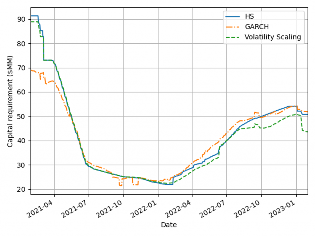
Figure 4: Capital charge for the VaR models measured on a diversified portfolio over the window 29/01/21 - 31/01/23.

Capital management efficiency

Pro-cyclicality of capital requirements is a common concern among regulators and practitioners. More stable requirements can improve banks’ capital management and planning. To measure models’ pro-cyclicality and efficiency, average capital charges and capital volatilities are compared for three concentrated asset class portfolios and a diversified market portfolio, as shown in Table 2. Volatility scaling results are better than the HS model across all portfolios, leading to lower capital charges, volatility and more efficient capital allocation. The GARCH model tends to underestimate high volatility and overestimate low volatility, as seen by the behaviour for the lowest volatility portfolio (Treasury).

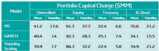
Table 2: Average capital requirement and capital volatility for each VaR model across a range of portfolios during the test period, 29/01/21 - 31/01/23.

Conclusions on VaR backtesting

Recent periods of market stress highlighted the need to challenge banks’ existing VaR models. Volatility scaling is an efficient method to enrich existing VaR methodologies, making them robust across a range of portfolios and volatility regimes.

VaR backtesting in a volatile market

Ensuring VaR models conform to VaR backtesting will be challenging with the recent period of stressed market conditions and rapid changes in market volatility. Banks will need to ensure that their VaR models are responsive to volatility clustering and tail events or enhance their existing methodology to cope. Failure to do so will result in additional overheads, with increased capital charges and excessive exceptions that can lead to additional regulatory scrutiny.

Enriching VaR Models with volatility scaling

Volatility scaling provides a simple extension of HS VaR that is robust and responsive to changes in market volatility. The model shows improved backtesting performance over both the HS and parametric (GARCH) VaR models. It is also robust for highly concentrated equity, treasury and bond portfolios, as seen in Table 3. Volatility scaling dampens pro-cyclicality of HS capital requirements, ensuring more efficient capital planning. The additional computational overhead is minimal and the implementation to enrich existing models is simple. Performance can be further improved with the use of hybrid models which incorporate volatility scaling approaches. These can utilise outlier detection to increase conservatism dynamically with increasingly volatile market conditions.

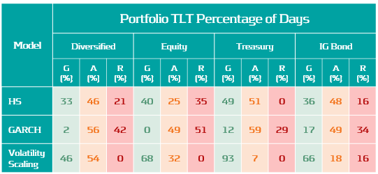
Table 3: Percentage of Green, Amber and Red traffic Lights test results for each VaR model across a range of portfolios for dates in the range: 13/02/19 - 31/01/23.

Zanders recommends

Banks should invest in making their VaR models more robust and reactive to ensure capital costs and the probability of exceptions are minimised. VaR models enriched with a volatility scaling approach should be considered among a suite of models to challenge existing VaR model methodologies. Methods similar to volatility scaling can also be applied to parametric and semi-parametric models. Outlier detection models can be used to identify changes in market regime as either feeder models or early warning signals for risk managers

Identifying the core of non-maturing deposits has become increasingly important for European banking Risk and ALM managers. This is especially true for retail banks whose funding mostly comprises deposits. The last years, the concept of core deposits was formalized by the Basel Committee and included in various regulatory standards. European regulators consider a disclosure requirement of the core NMD portion to regulators and possibly to public stakeholders. Despite these developments, a lot of banks still wonder: What is core deposits and how do I identify them?

FINDING FUNDING STABILITY: CORE PORTION OF DEPOSITS

Behavioural risk profiles for client deposits can be quite different per bank and portfolio. A portion of deposits can be stable in volume and price where other portions are volatile and sensitive to market rate changes. Before banks determine the behavioural (investment) profile for these funds, it should be analysed which deposits are suitable for long-term investment. This portion is often labelled as core deposits.

Basel standards define core deposits as balances that are highly likely to remain stable in terms of volume and are unlikely to reprice after interest rate changes. Behaviour models can vary a lot between (or even within) banks and are hard to compare. A simple metric such as the proportion of core deposits should make a comparison easier. The core breakdown alone should be sufficient to substantiate differences in the investment and risk profiles of deposits.

"A good definition of core deposit volume is tailored to banks’ deposit behavioural risk model."

Regulatory guidelines do not define the exact confidence level and horizon used for core analysis. Therefore banks need to formulate an interpretation of the regulatory guidance and set the assumptions on which their analysis is based. A good definition of core deposit volume is tailored to banks’ deposit behavioural risk model. Ideally, the core percentage can be calculated directly from behavioural model parameters. ALM and Risk managers should start with the review of internal behavioural models: how are volume and pricing stability modelled and how are they translated into investment restrictions?

SAVINGS MODELLING SERIES

This short article is part of the Savings Modelling Series, a series of articles covering five hot topics in NMD for banking risk management. The other articles in this series are:

• Non-maturing deposit model concepts for banking risk management
• Calibrating non-maturing deposit models: historic data or scenario analysis?
• The impact of savings rate floors on balance sheet management
• How ‘hidden savings’ dominate the risk profile of current accounts for banks

One of the puzzles for Risk and ALM managers at banks the last years has been determining the interest rate risk profile of non-maturing deposits. Banks need to substantiate modelling choices and parametrization of the deposit models to both internal and external validation and regulatory bodies. Traditionally, banks used historically observed relationships between behavioural deposit components and their drivers for the parametrization. Because of the low interest rate environment and outlook, historic data has lost (part of) its forecasting power. Alternatives such as forward-looking scenario analysis are considered by ALM and Risk functions, but what are the important focus points using this approach?

THE PROBLEM WITH USING HISTORICAL OBSERVATIONS

In traditional deposit models, it is difficult to capture the complex nature of deposit client rate and volume dynamics. On the one hand Risk and ALM managers believe that historical observations are not necessarily representative for the coming years. On the other hand it is hard to ignore observed behaviour, especially when future interest rates return to historic levels. To overcome these issues, model forecasts should be challenged by proper logical reasoning.

In many European markets, the degree to which customer deposit rates track market rates (repricing) has decreased over the last decade. Repricing decreased because many banks hesitate to lower rates below zero. Risk and ALM managers should analyse to what extent the historically decreasing repricing pattern is representative for the coming years and align with the banks’ pricing strategy. This discussion often involves the approval of senior management given the strategic relevance of the topic.

"Common sense and understanding deposit model dynamics are an integral part of the modelling process."

IMPROVING MODELS THROUGH FORWARD LOOKING INFORMATION

Common sense and understanding deposit model dynamics are an integral part of the modelling process (read our interview with ING experts here). Best practice deposit modelling includes forming a comprehensive set of interest rate scenarios that can be translated to a business strategy. To capture all possible future market developments, both downward and upward scenarios should be included. The slope of the interest rate scenarios can be adjusted to reflect gradual changes over time, or sudden steepening or flattening of the curve. Pricing experts should be consulted to determine the expected deposit rate developments over time for each of the interest rate scenarios. Deposit model parameters should be chosen in such a way that its estimations on average provide a best fit for the scenario analysis.

When going through this process in your own organisation, be aware that the effects of consulting pricing experts go both ways. Risk and ALM managers will improve deposit models by using forward-looking business opinion and the business’ understanding of the market will improve through model forecasts.

SAVINGS MODELLING SERIES

This short article is part of the Savings Modelling Series, a series of articles covering five hot topics in NMD for banking risk management. The other articles in this series are:

• How to determine core non-maturing deposit volume?
• Non-maturing deposit model concepts for banking risk management
• The impact of savings rate floors on balance sheet management
• How ‘hidden savings’ dominate the risk profile of current accounts for banks