A comparison between Survival Analysis and Migration Matrix Models

Navigating the complexities of loss modeling under IFRS 9 can be a daunting task, but with the right tools and knowledge, it can unlock opportunities for more accurate risk assessment and smarter decision-making.
This article provides a thorough comparison of the Survival Analysis and Migration Matrix approach for modeling losses under the internal ratings-based (IRB) approach and IFRS 9. The optimal approach depends on the bank’s situation, and this article highlights that there is no one-size-fits-all solution.
The focus of this read is on the probability of default (PD) component since IFRS 9 differs mainly with regards to the PD component as compared to the IRB Accords (Bank & Eder, 2021), and that most time and effort is given to this component.
Did you implement one approach and are you now wondering what the other approach would have meant for your IFRS 9 modeling? This article compares the two approaches of IFRS 9 modeling and can, thereby, support in answering the question if this approach is still the best approach for your institution.
Background
As of January 2018, banks reporting under IFRS faced the challenge of calculating their expected credit losses in a different way (IASB, 2023). Although IFRS 9 describes principles for calculating expected credit losses, it is not prescribed exactly how to calculate these losses. This in contrast to the IRB requirements, which prescribe how to calculate (un)expected credit losses. As a consequence, banks had to define the best approach to comply with the IFRS 9 requirements. Based on our experience, we look at two prominent approaches, namely: 1) Survival Analysis and 2) the Migration Matrix approach.
Survival Analysis approach
In the credit risk domain, the basic idea behind Survival Analysis is to estimate how long an obligor remains in the portfolio as of the moment of calculation. Survival Analysis models the time to default instead of the event of default and is therefore considered appropriate for modeling lifetime processes. This approach looks at the number of obligors that are at risk at a certain moment in time and the number of obligors that default during a certain period after that moment. Results are used to construct a cumulative distribution function of the time to default. Finally, the marginal probabilities can be obtained, which, after multiplication with the LGD and EAD, yield an estimation of the expected losses over the entire lifetime of a product.
Survival Analysis is particularly useful in addressing censoring in data, which occurs when the event of interest has not occurred yet for some individuals in the data set. Censoring is generally present in the realm of lifetime PD estimations of loans. Especially mortgage loan data is usually heavily censored due to its large maturity. Therefore, defaults may not yet have occurred in the relatively small data span available.
Various extensions of Survival Analysis are proposed in academic literature, enabling the inclusion of individual characteristics (covariates) that may or may not be varying over time, which is relevant if macroeconomic variables have to be included (PIT vs. TTC). For more background on Survival Analysis used for IFRS 9 PD modeling, please refer to Bank & Eder (2021).
We encounter Survival Analysis models frequently at institutions where credit risk portfolios are not (yet) modeled through advanced IRB models. This is due to the fact that IRB models, more specifically the PD models, form a very good basis for the Migration Matrix approach (see next paragraph). In the absence of IRB models, we observe that many institutions chose for the Survival Analysis approach in order to end with one single model, rather than two separate models.
One of the issues when using the Survival Analysis approach is that banks need to develop IRB and IFRS 9 PD models independently, which generally require different data sources and structures, and various methodologies for calculating PD. Consequently, inconsistencies in the estimated PD have been observed due to the utilization of different models and misalignment of IRB and IFRS 9 results. An example of such an inconsistency is an observed increase in estimated creditworthiness according to the IRB PD model, while the IFRS 9 PD decreases. Therefore, banks that chose to independently develop IRB and IFRS 9 PD models have regularly encountered difficulties in explaining these differences to regulators and management.
Migration Matrix approach
The existing infrastructure for estimating the expected loss for capital adequacy purposes, as prescribed by IRB, may be used as source to accommodate the use of IFRS 9 provision modeling. This finding is supported by a monitoring report published by the EBA, which indicates that 59% of the institutions examined have a dependence of their IFRS 9 on their IRB model (EBA, 2021).
IRB outcomes can be used as feeder model for IFRS 9 by utilizing migration matrices. Migration matrices can be established based on the existing rating system, i.e. the IRB rating system used for capital requirements. Each of these ratings can be seen as a state of a Markov Chain, for which the migration probabilities are illustrated in a Migration Matrix. Consequently, along with the probability of default, transformations in creditworthiness may also be observed. A convenient feature of this approach is the ability to extend the horizon on which the PD is estimated by straightforward matrix multiplication. This is especially useful for complying with both IRB and IFRS 9 regulations, where 12-month and multi-period predictions are required, respectively.
Estimating the PD under IRB and IFRS 9 comes with an additional challenge; PDs for capital are required to be Through-The-Cycle (TTC), while IFRS 9 requires them to be Point-In-Time (PIT), depending on macro-economic conditions. A popular model that facilitates the conversion between these two objectives is the Single Factor Vasicek Model (Vasicek, 2002).This model shocks the TTC Migration Matrix with a single risk factor, Z, which is dependent on macroeconomic risk drivers. Consequently, PIT migration matrices are attained, conditional on a future value of Z. Forecasting Z multiple periods ahead enables one to create a series of PIT transition matrices that can be viewed as a time-inhomogeneous Markov Chain. Subsequently, lifetime estimates of the PDs can be calculated by multiplying these matrices.
One of the main issues in applying the migration matrix approach is that you cannot redevelop or recalibrate IRB and IFRS 9 models in parallel. You require to first finish the IRB model before you finish your IFRS 9 model.
Comparison Migration Matrix approach and Survival Analysis
We will now zoom in on the differences between the two approaches mentioned above. This doesn’t imply that these approaches do not share characteristics. Commonalities are, amongst other, that both approaches yield an estimate for future PD, can incorporate macro-economic expectations and are often used during stress test exercises. Table 1 presents a summary of the key features of both the Migration Matrix approach and Survival Analysis, and their interrelationships. The Migration Matrix approach is characterized by its use of a unified PD structure. When estimating different PDs for IRB and IFRS 9, this allows for a simpler explanation on why these differ. Survival Analysis offers the advantage of estimating PD on a per-obligor basis, as opposed to the Migration Matrix approach, which calculates the average PD per rating category. Accordingly, the Migration Matrix approach operates under the assumption that obligors within the same rating category possess similar average PDs over the long term which might not be true.
Whilst the above constitute the primary differences, the two approaches demonstrate many variations across the diverse categories in Table 1. Accordingly, each situation may require a distinct optimal approach implying the absence of a universal best practice.
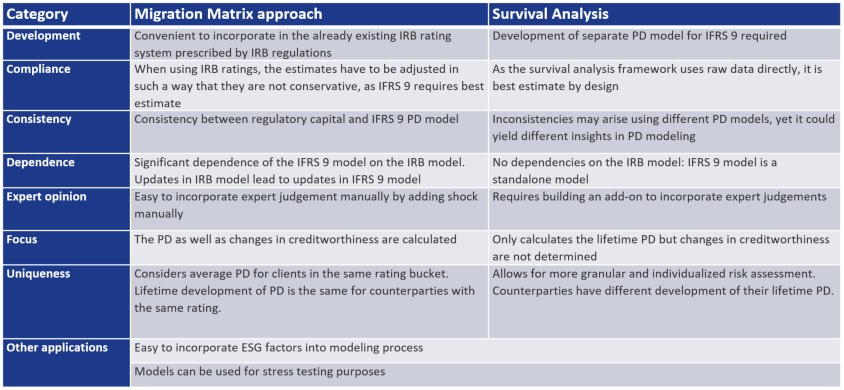
Table 1: Migration Matrix approach vs Survival Analysis
The table of differences indicates that selecting the best approach can be challenging as both approaches have their respective advantages and disadvantages. Therefore, there is no one-size-fits-all solution, and the optimal choice depends on the specific institution’s situation. Fortunately, our experts in this field are available and eager to collaborate with you in identifying and implementing the best possible modeling approach for your institution.
References:
Bank, M., & Eder, B. (2021). A review on the Probability of Default for IFRS 9. Available at SSRN 3981339.
Gae-Carrasco, C. (2015). IFRS 9 Will Significantly Impact Banks’ Provisions and Financial Statements. Moody’s Analytics Risk Perspectives.
IASB (2023). IFRS 9 Financial Instruments. Retrieved from https://www.ifrs.org/issued-standards/list-of-standards/ifrs-9-financial-instruments/
Vasicek, O. (2002). The distribution of loan portfolio value. Risk, 160-162.
-
Margin of Conservatism Explained: Reducing Capital Inflation in IRB Models

-
Cash Is King Again: Why real-time liquidity is the new strategic advantage

-
CEO Statement: Delivering Financial Performance When It Counts

-
The Digital Agenda Has Increased the Cybercrime and Fraud Threat Landscape – It’s Now Critical for Corporate Treasury to Build Resilience

-
The New Rails: How Stablecoins Are Redefining Cross-Border Payments for Corporate Treasury

-
Risk Mitigation Accounting (RMA) Exposure Draft amending IFRS9: Key Impacts and Practical Challenges

-
Optimizing the Valuation Processes in Modern Banking: A Strategic Approach to Efficiency, Consistency, and Cost Reduction

-
Intra-Group Loans Transfer Pricing: What’s Important in 2026?

-
A Roadmap for Banks to Geopolitical Risk Taxonomy

-
Geopolitical Risk and the ECB 2026 Reverse Stress Test: Mapping Failure Pathways Before It’s Too Late