Using Capital Attribution to Understand Your FRTB Capital Requirements

As FRTB tightens the screws on capital requirements, banks must get smart about capital attribution.
Industry surveys show that FRTB may lead to a 60% increase in regulatory market risk capital requirements, placing significant pressure on banks. As regulatory market risk capital requirements rise, it is imperative that banks employ robust techniques to effectively understand and manage the drivers of capital. However, isolating these drivers can be challenging and time-consuming, often relying on inefficient and manual techniques. Capital attribution techniques provide banks with a solution by automating the analysis and understanding of capital drivers, enhancing their efficiency and effectiveness in managing capital requirements.
In this article, we share our insights on capital attribution techniques and use a simulated example to compare the performance of several approaches.
The benefits of capital attribution
FRTB capital calculations require large amounts of data which can be difficult to verify. Banks often use manual processes to find the drivers of the capital, which can be inefficient and inaccurate. Capital attribution provides a quantification of risk drivers, attributing how each sub-portfolio contributes to the total capital charge. The ability to quantify capital to various sub-portfolios is important for several reasons:

An overview of approaches
There are several existing capital attribution approaches that can be used. For banks to select the best approach for their individual circumstances and requirements, the following factors should be considered:
- Full Allocation: The sum of individual capital attributions should equal the total capital requirements,
- Accounts for Diversification: The interactions with other sub-portfolios should be accounted for,
- Intuitive Results: The results should be easy to understand and explain.
In Table 1, we summarize the above factors for the most common attribution methodologies and provide our insights on each methodology.

Table 1: Comparison of common capital attribution methodologies.
Comparison of approaches: A simulated example
To demonstrate the different performance characteristics of each of the allocation methodologies, we present a simulated example using three sub-portfolios and VaR as a capital measure. In this example, although each of the sub-portfolios have the same distribution of P&Ls, they have different correlations:
- Sub-portfolio B has a low positive correlation with A and a low negative correlation with C,
- Sub-portfolios A and C are negatively correlated with each other.
These correlations can be seen in Figure 1, which shows the simulated P&Ls for the three sub-portfolios.

Figure 1: Simulated P&L for the three simulated sub-portfolios: A, B and C.
The capital allocation results are shown below in Figure 2. Each approach produces an estimate for the individual sub-portfolio capital allocations and the sum of the sub-portfolio capitals. The dotted line indicates the total capital requirement for the entire portfolio.

Figure 2: Comparison of capital allocation methodologies for the three simulated sub-portfolios: A, B and C. The total capital requirement for the entire portfolio is given by the dotted line.
Zanders’ verdict
From Figure 2, we see that several results do not show this attribution profile. For the Standalone and Scaled Standalone approaches, the capital is attributed approximately equally between the sub-portfolios. The Marginal and Scaled Marginal approaches include some estimates with negative capital attribution. In some cases, we also see that the estimate for the sum of the capital attributions does not equal the portfolio capital.
The Shapley method is the only method that attributes capital exactly as expected. The Euler method also generates results that are very similar to Shapley, however, it allocates almost identical capital in sub-portfolios A and C.
In practice, the choice of methodology is dependent on the number of sub-portfolios. For a small number of sub-portfolios (e.g. attribution at the level of business areas) the Shapley method will result with the most intuitive and accurate results. For a large number of sub-portfolios (e.g. attribution at the trade level), the Shapley method may prove to be computationally expensive. As such, for FRTB calculations, we recommend using the Euler method as it is a good compromise between accuracy and cost of computation.
Conclusion
Understanding and implementing effective capital attribution methodologies is crucial for banks, particularly given the increased future capital requirements brought about by FRTB. Implementing a robust capital attribution methodology enhances a bank's overall risk management framework and supports both regulatory compliance and strategic planning. Using our simulated example, we have demonstrated that the Euler method is the most practical approach for FRTB calculations. Banks should anticipate capital attribution issues due to FRTB’s capital increases and develop reliable attribution engines to ensure future financial stability.
For banks looking to anticipate capital attribution issues and potentially mitigate FRTB’s capital increases, Zanders can help develop reliable attribution engines to ensure future financial stability. Please contact Dilbagh Kalsi (Partner) or Robert Pullman (Senior Manager) for more information.
PLA and the RFET: A Perfect FRTB Storm

Banks face challenges with PLA and RFET under FRTB; a unified approach can reduce capital requirements and improve outcomes by addressing shared risk factors.
Despite the several global delays to FRTB go-live, many banks are still struggling to be prepared for the implementation of profit and loss attribution (PLA) and the risk factor eligibility test (RFET). As both tests have the potential to considerably increase capital requirements, they are high on the agenda for most banks which are attempting to use the internal models approach (IMA).
In this article, we explore the difficulties with both tests and also highlight some underlying similarities. By leveraging these similarities to develop a unified PLA and RFET system, we describe how PLA and RFET failures can be avoided to reduce the potential capital requirements for IMA banks.
Difficulties with PLA
Since its introduction into the FRTB framework by the Basel Committee on Banking Supervision (BCBS), the PLA test has been a consistent cause for concern for banks attempting to use the IMA. The test is designed to ensure that Front Office (FO) and Risk P&Ls are sufficiently aligned. As such, it ensures that banks’ internal models for market risk accurately reflect the risk they are exposed to. To assess this alignment, the PLA test compares the Hypothetical P&L (HPL) from the FO with the risk-theoretical P&L (RTPL) from Risk using two statistical tests - the Spearman correlation and the Kolmogorov-Smirnov (KS) test.
There are potentially significant consequences of trading desks not passing the test. At best, the desk will incur capital add-ons. At worst, the desk will be forced to use the more punitive standardised approach (SA), which may increase capital requirements even more.
There are several difficulties with PLA:
- No existing systems: As the test has never before been a regulatory requirement, many banks do not have suitable existing systems and processes which can be leveraged to identify the causes of PLA failures. Although the KS and Spearman tests are easy to implement, isolating the causes of PLA failures can be difficult.
- Risk factor mapping: Banks often do not have accurate and reliable mapping between the risk factors in the FO and Risk models. Remediation of the inaccurate mapping can often be a slow and manual process, making it extremely difficult to identify the risk factors which are causing the PLA failure.
- Data inconsistency: As the data feeds between Risk and FO models can be different, there can be a large number of potential causes of P&L differences. Even small differences in data granularity, convexity capture or even holiday calendars can cause misalignments which may result in PLA failures.
- Hedged portfolios: Well-hedged portfolios often find it more challenging to pass the PLA test. When portfolios are hedged, the total P&L of the portfolio is reduced, leading to a larger relative error than that of an unhedged portfolio, potentially causing PLA failures. You can read more about this topic on our other blog post – ‘To Hedge or Not to Hedge: Navigating the Catch-22 of FRTB’s PLA Test’
Issues with the RFET
The RFET ensures that all risk factors in the internal model have a minimum level of liquidity and enough market data to be accurately used. Liquidity is measured by the number of real price observations which have been observed in the past 12 months. Any risk factors that do not meet the minimum liquidity standards outlined in FRTB are known as non-modellable risk factors (NMRFs). Similar to the consequences of failing the PLA test and having to use the SA, NMRFs must use the more conservative stressed expected shortfall (SES) capital calculations, leading to higher capital requirements. Research shows that NMRFs can account for over 30% of capital requirements, making them one of the most punitive drivers of increased capital within the IMA. The impact of NMRFs is often considered to be disproportionately large and also unpredictable.
There are several difficulties with the RFET:
- Wide scope: The RFET requires all risk factors to be collected across multiple desks and systems. Mapping instruments to risk factors can be a complicated and lengthy process. Consequently, implementing and operationalizing the RFET can be difficult.
- Diversification benefit: Modellable risk factors are capitalised using the expected shortfall (ES) which allows for diversification benefits. However, NMRFs are capitalised using the stressed expected shortfall (SES) which does not provide the same benefits, resulting in larger capital.
- Proxy development: Although proxies can be used to overcome a lack of data, developing them can be time-consuming and require considerable effort. Determining proxies requires exploratory work which often has uncertain outcomes. Furthermore, all proxies need to be validated and justified to the regulator.
- Vendor data: It can be difficult for banks to quantify the cost benefit of purchasing external data to increase the number of real price observations versus the cost of more NMRFs. Ultimately, the result of the RFET is based on a bank’s access to real price observation data. Although two banks may have identical exposures and risk, they may have completely different capital requirements due to their access to the correct data.
The interconnectedness of both tests
Despite their individual difficulties, there are a number of similarities between PLA and the RFET which can be leveraged to ensure efficient implementation of the IMA:
- Although PLA is performed at the desk-level, the underlying risk factors are the same as those which are used for the RFET.
- Both tests potentially impact the ES model as the PLA/RFET outcomes may instigate modifications to the model in order to improve the results. For example, any changes in data source to increase the liquidity of NMRFs (which is a common way to overcome RFET issues) would require PLA to be rerun.
- Ultimately, if any changes are made to the underlying risk factors, both tests must be performed again.
- Hence, although they are relatively simple tests (Spearman Correlation and KS, and a count of real price observations for the RFET), banks must develop a reliable architecture to dynamically change risk factors and efficiently rerun PLA and RFET tests.
Zanders’ recommendation
As they greatly impact one another, a unified system allows both components to be run together. Due to their interdependencies, a unified PLA-RFET system makes it easier for banks to dynamically modify risk factors and improve results for both tests.
- In order to truly have a unified PLA-RFET system, the PLA results must also be brought down to the risk factor level. This is done by understanding and quantifying which risk factors are causing the discrepancies between RTPL and HPL and causing poor PLA statistics. More information about this can be found in our other blog post ‘FRTB: Profit and Loss Attribution (PLA) Analytics’.
- Once the risk factors causing PLA failures have been identified, a unified approach can prioritise risk factors which, if remediated, improve PLA statistics and also efficiently reduce NMRF SES capitalisation.
Conclusion
While PLA is crucial for IMA approval, it presents numerous operational and technical challenges. Similarly, the RFET introduces additional complexities by enforcing strict liquidity and data standards for risk factors, with failing risk factors subject to harsher capital treatments. The interconnected nature of both tests highlights the need for a cohesive strategy, where adjustments to one test can directly influence outcomes in the other. Ultimately, banks need to invest in robust systems that allow for dynamic adjustments to risk factors and efficient reruns of both tests. A unified PLA-RFET approach can streamline processes, reduce capital penalties, and improve test results by focusing on the underlying risk factors common to both assessments.
For more information about this topic and how Zanders can help you design and implement a unified PLA and RFET system, please contact Dilbagh Kalsi (Partner) or Hardial Kalsi (Manager).
To Hedge or Not to Hedge: Navigating the Catch-22 of FRTB’s PLA Test

FRTB PLA’s catch-22: hedging, used to reduce a portfolio’s risk, may actually increase the likelihood of failing the PLA test.
Profit and loss attribution (PLA) is a critical component of FRTB’s internal models approach (IMA), ensuring alignment between Front Office (FO) and Risk models. The consequences of a PLA test failure can be severe, with desks forced to use the more punitive standardised approach (SA), resulting in a considerable increase in capital charges. The introduction of the PLA test has sparked controversy as it appears to disincentivise the use of hedging. Well-hedged portfolios, which reduce risk and variability in a portfolio's P&L, often find it more challenging to pass the PLA test compared to riskier, unhedged portfolios.
In this article, we dig deeper into the issues surrounding hedging with the PLA test and provide solutions to help improve the chances of passing the test.
The problem with performing PLA on hedged portfolios
The PLA test measures the compatibility of the risk theoretical P&L (RTPL), produced by Risk, with the hypothetical P&L (HPL) produced by the FO. This is achieved by measuring the Spearman correlation and Kolmogorov–Smirnov (KS) test statistic on 250 days of historical RTPLs and HPLs for each trading desk. Based on the results of these tests, desks are assigned a traffic light test (TLT) zone categorisation, defined below. The final PLA result is the worst TLT zone of the two tests.
| TLT Zone | Spearman Correlation | KS Test |
| Green | > 0.80 | < 0.09 |
| Amber | < 0.80 | > 0.09 |
| Red | < 0.70 | > 0.12 |
The impact of TLT zones
The impact of a desk’s PLA results depends on which TLT zone it has been assigned:
- Green zone: Desks are free to calculate their capital requirements using the IMA.
- Amber zone: Desks are required to pay a capital surcharge, which can lead to a considerable increase in their capital requirements.
- Red zone: Desks must calculate their capital requirements using the SA, which can lead to a significant increase in their capital.
Red and Amber desks must also satisfy 12-month backtesting exception requirements before they can return to the green zone.
Why are hedged portfolios more susceptible to failing the PLA test?
Due to modelling and data differences, we typically expect there to exist a small difference (error) between RTPLs and HPLs. For unhedged portfolios, the total P&L is typically much larger than this error, resulting in a small relative error. When portfolios are hedged, the total P&L of the portfolio is reduced, leading to a larger relative error than that of an unhedged portfolio. This is illustrated in Figure 1, which shows how for the same modelling error, a significantly different relative error can be observed, depending on the degree of hedging of the portfolios.
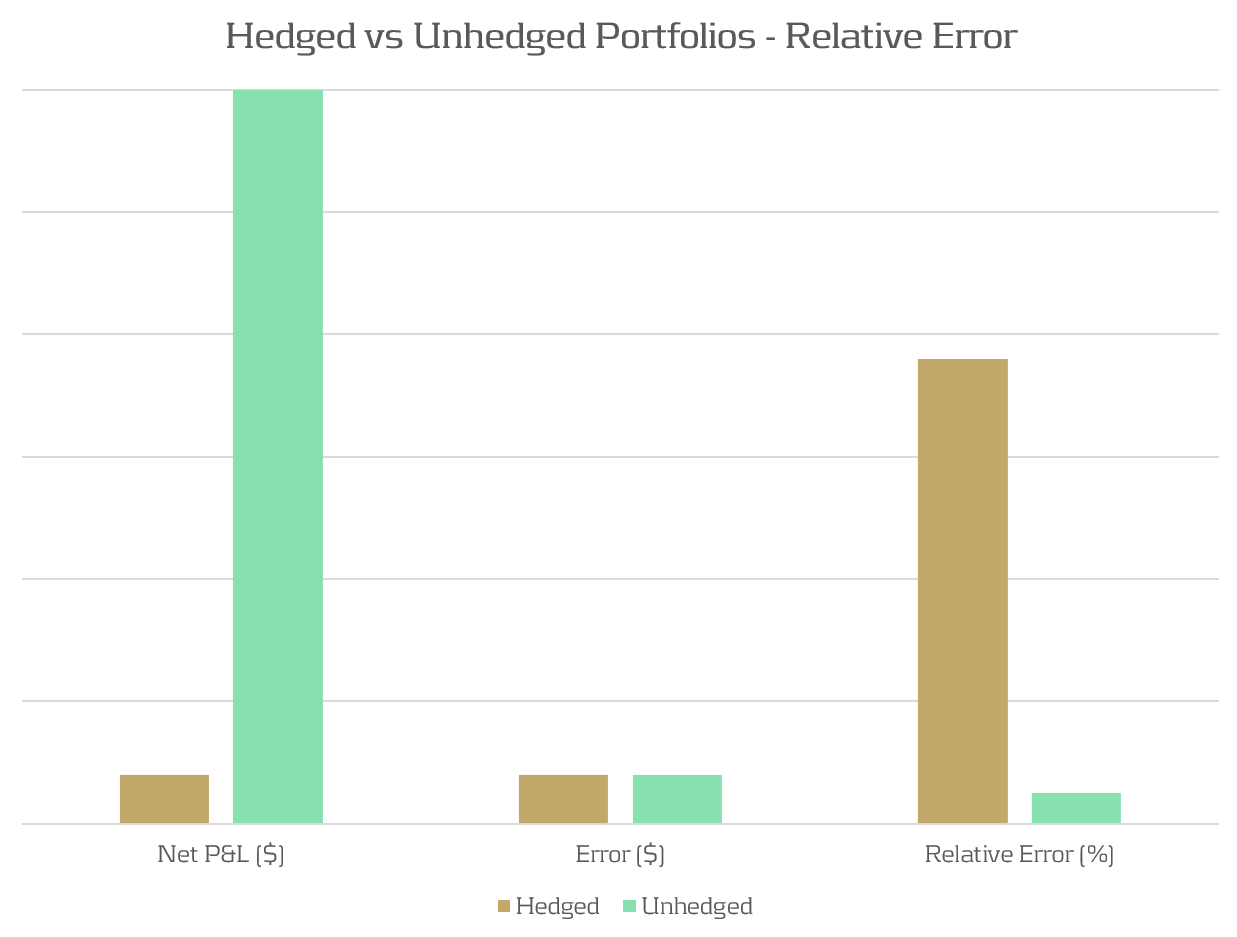
Figure 1: The relative P&L error can be significantly different between hedged and unhedged portfolios which have the same absolute error.
Demonstration: A delta-hedged option portfolio
Portfolio and simulation
To demonstrate the PLA hedging issue, we examine a simulated example of a desk with long put positions, hedged by a variable quantity of the underlying stock. In this example, the portfolio consists of 100 long puts and between 0 and 100 of the underlying stock as a hedge against the put positions.
To emulate the differences in pricing models between Risk and FO, a closed form solution is used to compute HPLs and a Monte Carlo pricing methodology is used for RTPLs. This produces a sufficiently small pricing error, such that the options and stock positions would comfortably pass the PLA test if they were held in separate portfolios. The P&Ls are obtained by repricing 250 scenarios of a Monte Carlo simulation of the underling risk factors.
The outcome
The results in Figure 2 show the PLA results for the two statistical tests against the total hedge ratio (the ratio between stock position delta and put position delta). The TLT zones are represented by the green, amber, and red shaded regions. This shows that the test statistics can vary quite considerably depending on the degree of hedging, with the KS test statistic entering the amber and red TLT zones for even a limited degree of hedging. The Spearman correlation is not as sensitive to the hedge ratio, but the statistic worsens as the hedging ratio approaches 100%.
Although the portfolio comfortably passes the PLA test when unhedged, it fails when hedged. Hence, quite surprisingly, hedging strategies used by banks to reduce risk may in fact be penalised by the regulator and increase capital requirements. Furthermore, failing desks would also need to satisfy 12-month PLA and backtesting requirements to return to the IMA.
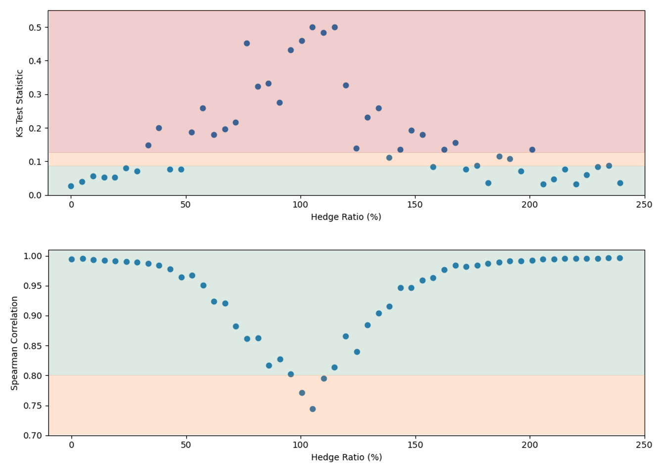
Figure 2: The KS (top) and Spearman correlation (bottom) statistics for an example portfolio of 100 long puts and between 0 and 100 shares of the underlying stock. The hedge ratio is defined as the ratio between stock position delta and put position delta. The green, amber, and red shading represent the TLT zones.
Solutions for Hedged Portfolios
Reducing the impact of hedged portfolios
As demonstrated, some trading desks with well-hedged positions may find themselves losing IMA eligibility due to poor performance in the PLA test. However, the following strategies can be used to reduce the possibility of failures:
- Model Alignment: Ensure the modelling methodologies of risk factors and instrument pricing are consistent between FO and Risk.
- Data Alignment: Ensure that the data sourced for FO and Risk are aligned and are of similar quality and granularity.
- Risk Enhancements: Improve the sophistication of Risk pricing models to better incorporate the subtilities of the FO pricer. This may require pricing optimisations and high-performance computing.
- Proactive Monitoring: Develop ongoing monitoring frameworks to identify and remediate P&L issues early. We provide more insights on the development of PLA analytics here.
Will regulatory policy change be required?
It is clear that the current PLA regulation does not correctly account for the effects of hedging on the PLA test statistics, resulting in hedged portfolios being penalised. As banks move towards implementing FRTB IMA, regulators should reflect on the impact of the current PLA implementation and consider providing exemptions for hedged portfolios or, alternatively, a fundamental modification of the PLA test.
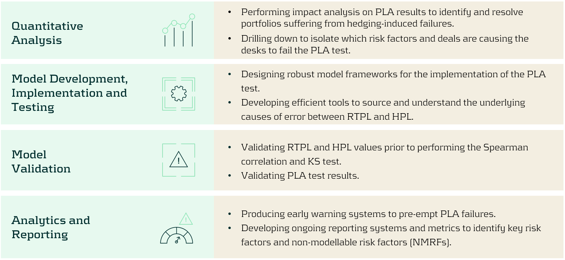
Zanders’ services
Zanders is ideally suited to helping clients develop models and implement FRTB workstreams. Below, we highlight a selection of the services we provide to implement, analyse, and improve PLA test results:
Conclusion
The PLA test under FRTB can disproportionately penalise well-hedged portfolios, forcing trading desks to adopt the more punitive SA. This effect is exacerbated by complex hedging strategies and non-linear instruments, which introduce additional model risks and potential discrepancies. To mitigate these issues, it is essential banks take steps to align their pricing models and data between FO and Risk. Implementing robust analytics frameworks to identify P&L misalignments is critical to quicky and proactively solve PLA problems. Zanders offers comprehensive services to help banks navigate the complexities of PLA and optimise their regulatory capital requirements.
For more information on this topic, contact Dilbagh Kalsi (Partner) or Hardial Kalsi (Manager).


