Roundtable ‘Climate Scenario Design & Stress Testing’ recap

On Thursday 15 June 2023, Zanders hosted a roundtable on ‘Climate Scenario Design & Stress Testing’. This article discusses our view on the topic and highlights key insights from the roundtable.
On Thursday 15 June 2023, Zanders hosted a roundtable on ‘Climate Scenario Design & Stress Testing’. In our head office in Utrecht, we welcomed risk managers from several Dutch banks. This article discusses our view on the topic and highlights key insights from the roundtable.
In recent years, many banks took their first steps in the integration of climate and environmental (C&E) risks into their risk management frameworks. The initial work on climate-related risk modeling often took the form of scenario analysis and stress testing. For example, as part of the Internal Capital Adequacy Assessment Process (ICAAP) or by participating in the 2022 Climate Stress Test by the European Central Bank (ECB). To comply with the ECB’s expectations on C&E risks, banks are actively exploring methodologies and data sources for adequate climate scenario design and stress testing. The ECB requires that banks will meet their expectations on this topic by 31 December 2024.
Our view
We believe that banks should start early with climate stress testing, but in a manageable and pragmatic way. Banks can then improve their methodologies and extend their scope over time. This allows for a gradual development of knowledge, data and methodologies within all relevant Risk teams. Zanders has identified the following steps in the process of climate scenario design and stress testing:
- Step 1: Scenario selection
A bank has to select appropriate (climate) scenarios based on the bank’s climate risk materiality assessment. Important to consider in this phase is the purpose for which the scenarios will be used, whether the scenarios are in line with scientific pathways, and whether they account for different policy outcomes (like an early or late transition to a sustainable economy).
- Step 2: Scope and variable definition
An appropriate scope must then be selected and appropriate variables defined. For example, banks need to determine which portfolios to take in scope, which time horizons to include, select the granularity of the output, the right level of stress, and which climate- and macro-economic variables to consider.
- Step 3: Methodology
Then, the bank needs to develop methodologies to calculate the impact of the scenarios. There are no one-size-fits-all approaches and often a combination of different qualitative and quantitative methodologies is needed. We recommend that the climate stress test approach be initially simple and to focus on material exposures.
- Step 4: Results
It is important to use the results of the scenario analysis in the relevant risk and business processes. The results can be used for the bank’s risk appetite and strategy. The results can also help to create awareness and understanding among internal stakeholders, and support external disclosures and compliance.
- Step 5: Stress testing framework
Finally, banks should establish minimum standards for climate scenario design and stress testing. This framework should include, amongst others, policies and processes for data collection from different sources, how adequate knowledge and resources are ensured, and how the scenarios are kept up-to-date with the latest market developments.
Key insights
Prior to the roundtable, participants filled in a survey related to the progress, scope and challenges on climate risk stress testing. The key insights presented below are based on the results of this survey, together with the outcomes of the discussion thereafter.
The financial sector has advanced with several aspects around integrating climate risks in risk management over the past year. This was recognized by all participants, as they had all performed some form of climate risk stress testing. The scope of the stress testing, however, was relatively limited in some cases. For example, all participants considered credit risk in their climate risk scenario with many also including market risk. Only a limited number of participants took other risk types into account.
Furthermore, all participants assessed the short-term impact (up to 3 years) of the climate scenarios, whereas only around 40% and 10% assessed the impact on the medium term (3 to 10 years) and long term (>10 years), respectively. This is probably related to the fact that all participants used climate scenarios in their ICAAP, which typically covers a three-year horizon. The second most mentioned use for the climate scenarios, after the ICAAP, was the risk identification & materiality analysis. A smaller percentage of participants also used the climate scenarios for business strategy setting, ILAAP and portfolio management.
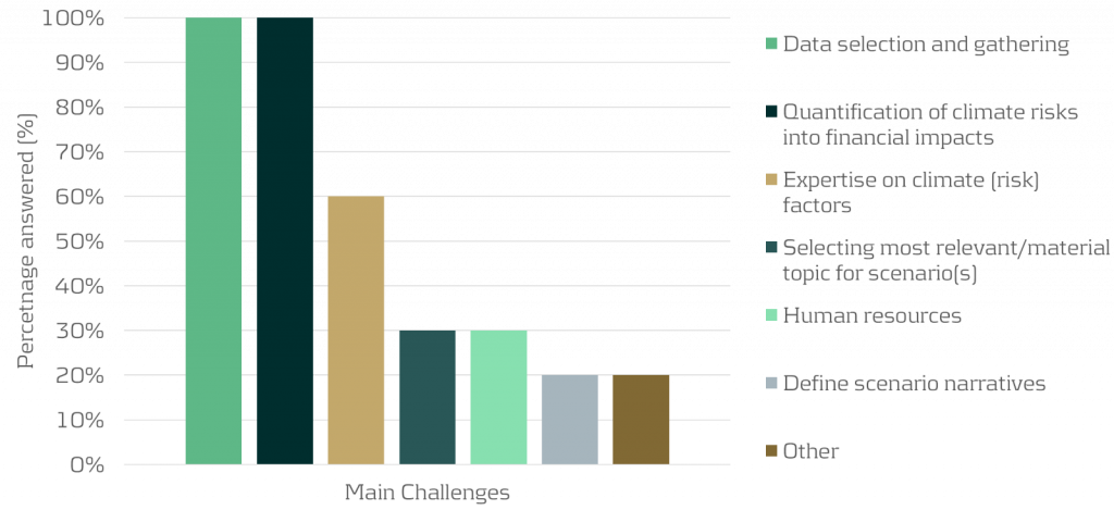
The two topics that were unanimously mentioned as the main challenges in climate risk stress testing are data selection and gathering, and the quantification of climate risks into financial impacts, as shown in the graph below:
- Insight 1: Assessing impact of climate risk beyond the short-term very much increases the complexity and uncertainty of the exercise
The participants indicated that climate stress testing beyond the short-term horizon (beyond 3 to 5 years) is very difficult. Beyond that horizon, the complexity of the (climate) scenarios increases materially due to uncertainties of clients’ transition plans, the bank’s own transition plan and climate strategy (e.g., related to pricing and client acceptance policies), and climate policies and actions from governments and regulators. Taking the transition plans of clients into account on a granular level is especially difficult when there is a large number of counterparties. There are no clear solutions to this. Some ideas that take longer-term effects into account were floated, such as adjusting the current valuation of various assets by translating future climate impact on assets into a net present value of impact or by taking climate impacts into account in the long-term macro-economic scenarios of IFRS9 models.
- Insight 2: Whether to use a top-down or bottom-up approach depends on the circumstances
It was discussed whether a bottom-up stress test for climate scenarios is preferable to a top-down stress test. The consensus was that this depends on the circumstances, for example:- Physical risks are asset- and location-specific; one street may flood but not the next. So, in that case a bottom-up assessment may be necessary for a more granular approach. On the other hand, for transition risks, less granularity might be sufficient as transition policies are defined on national or even supranational level, and trends and developments often materialize on sector-level. In those cases, a top-down type of analysis could be sufficient.
- If the climate stress test is used to get a general overview of where risks are concentrated, a top-down analysis may be appropriate. However, if it is used to steer clients, a more granular, bottom-up approach may be needed.
- A bottom-up approach could also be more suitable for longer-term scenarios as it allows to include counterparty-specific transition plans. For more short-term scenarios, a sector average may be sufficient, considering that there will be less transition during this period.
- Insight 3: Translating the results of climate risk stress testing into concrete actions is challenging
The results of the stress test can be used to further integrate climate risk into risk management processes such as materiality assessment, risk appetite, pricing, and client acceptance. Most participants, however, were still hesitant to link any binding actions to the results, such as setting risk limits (e.g., limiting exposures to a certain sector), adjusting client acceptance, or amending pricing policies. However, the ECB does require banks to consider climate impacts in these processes. The most mentioned uses of the climate risk stress testing results were risk identification & materiality assessments and risk monitoring.
Conclusion
Most banks have taken first steps in relation to climate scenario design and stress testing. However, many challenges still remain, for example around data selection and quantification methodologies. Efforts by banks, regulators and the market in general are required to overcome these challenges.
Zanders has already supported several banks with climate scenario design and stress testing. This includes the creation of a climate scenario design framework, the definition of climate scenarios, and by quantifying climate risk impacts for the ICAAP. Next to that, we have performed research on modeling approaches that can be used to quantify the impact of transition and physical risks. If you are interested to know how we can help your organization with this, please reach out to Marije Wiersma.
Performance of Dutch banks in the 2023 EBA stress test

At the end of July, the European Banking Authority (EBA) released the results on the latest installment of the EU-wide stress test that is performed every two years.
Seventy banks have been considered, which is an increase of twenty banks compared to the previous exercise. The portfolios of the participating banks contain around three quarters of all EU banking assets (Euro and non-Euro).
Interested in how the four Dutch banks participating in this EBA stress test exercise performed? In this short note we compare them with the EU average as represented in the results published [1].
General comments
The general conclusion from the EU wide stress test results is that EU banks seem sufficiently capitalized. We quote the main 5 points as highlighted in the EBA press release [1]:
- The results of the 2023 EU-wide stress test show that European banks remain resilient under an adverse scenario which combines a severe EU and global recession, increasing interest rates and higher credit spreads.
- This resilience of EU banks partly reflects a solid capital position at the start of the exercise, with an average fully-loaded CET1 ratio of 15% which allows banks to withstand the capital depletion under the adverse scenario.
- The capital depletion under the adverse stress test scenario is 459 bps, resulting in a fully loaded CET1 ratio at the end of the scenario of 10.4%. Higher earnings and better asset quality at the beginning of the 2023 both help moderate capital depletion under the adverse scenario.
- Despite combined losses of EUR 496bn, EU banks remain sufficiently apitalized to continue to support the economy also in times of severe stress.
- The high current level of macroeconomic uncertainty shows however the importance of remaining vigilant and that both supervisors and banks should be prepared for a possible worsening of economic conditions.
For further details we refer to the full EBA report [1].
Dutch banks
Making the case for transparency across the banking sector, the EBA has released a detailed breakdown of relevant figures for each individual bank. We use some of this data to gain further insight into the performance of the main Dutch banks versus the EU average.
CET1 ratios
Using the data presented by EBA [2], we display the evolution of the fully loaded CET1 ratio for the four banks versus the average over all EU banks in the figure below. The four Dutch banks are: ING, Rabobank, ABN AMRO and de Volksbank, ordered by size.
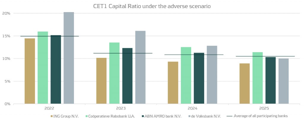
From the figure, we observe the following:
- Compared to the average EU-wide CET1 ratio (indicated by the horizontal lines in the graph above), it can be observed that three out of four of the banks are very close to the EU average.
- For the average EU wide CET1 ratio we observe a significant drop from year 1 to year 2, while for the Dutch banks the impact of the stress is more spread out over the full scenario horizon.
- The impact after year 4 of the stress horizon is more severe than the EU average for three out of four of the Dutch banks.
Evolution of retail mortgages during adverse scenario
The most important product the four Dutch banks have in common are the retail mortgages. We look at the evolution of the retail mortgage portfolios of the Dutch banks compared to the EU average. Using EBA data provided [2], we summarize this in the following chart:
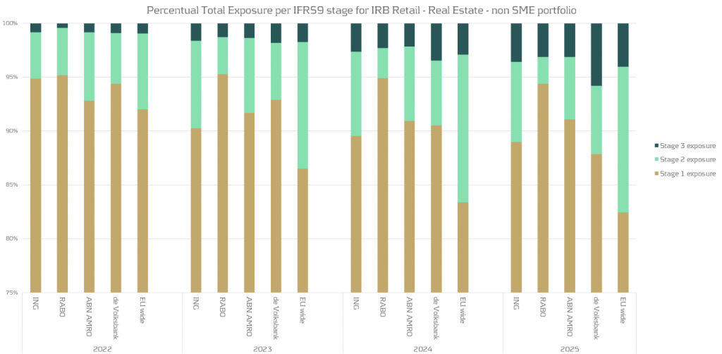
Based on the analysis above , we observe:
- There is a noticeable variation between the banks regarding the migrations between the IFRS stages.
- Compared to the EU average there are much less mortgages with a significant increase in credit risk (migrations to IFRS stage 2) for the Dutch banks. For some banks the percentage of loans in stage 2 is stable or even decreases.
Conclusion
This short note gives some indication of specifics of the 2023 EBA stress applied to the four main Dutch banks.
Should you wish to go deeper into this subject, Zanders has both the expertise and track record to assist financial organisations with all aspects of stress testing. Please get in touch.
References
FRTB: Profit and Loss Attribution (PLA) Analytics

At the end of July, the European Banking Authority (EBA) released the results on the latest installment of the EU-wide stress test that is performed every two years.
Under FRTB regulation, PLA requires banks to assess the similarity between Front Office (FO) and Risk P&L (HPL and RTPL) on a quarterly basis. Desks which do not pass PLA incur capital surcharges or may, in more severe cases, be required to use the more conservative FRTB standardised approach (SA).
What is the purpose of PLA?
PLA ensures that the FO and Risk P&Ls are sufficiently aligned with one another at the desk level. The FO HPL is compared with the Risk RTPL using two statistical tests. The tests measure the materiality of any simplifications in a bank’s Risk model compared with the FO systems. In order to use the Internal Models Approach (IMA), FRTB requires each trading desk to pass the PLA statistical tests. Although the implementation of PLA begins on the date that the IMA capital requirement becomes effective, banks must provide a one-year PLA test report to confirm the quality of the model.
Which statistical measures are used?
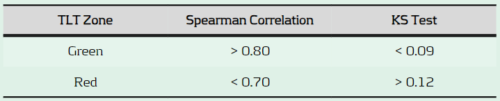
PLA is performed using the Spearman Correlation and the Kolmogorov-Smirnov (KS) test using the most recent 250 days of historical RTPL and HPL. Depending on the results, each desk is assigned a traffic light test (TLT) zone (see below), where amber desks are those which are allocated to neither red or green.
What are the consequences of failing PLA?
Capital increase: Desks in the red zone are not permitted to use the IMA and must instead use the more conservative SA, which has higher capital requirements. Amber desks can use the IMA but must pay a capital surcharge until the issues are remediated.
Difficulty with returning to IMA: Desks which are in the amber or red zone must satisfy statistical green zone requirements and 12-month backtesting requirements before they can be eligible to use the IMA again.
What are some of the key reasons for PLA failure?
Data issues: Data proxies are often used within Risk if there is a lack of data available for FO risk factors. Poor or outdated proxies can decrease the accuracy of RTPL produced by the Risk model. The source, timing and granularity also often differs between FO and Risk data.
Missing risk factors: Missing risk factors in the Risk model are a common cause of PLA failures. Inaccurate RTPL values caused by missing risk factors can cause discrepancies between FO and Risk P&Ls and lead to PLA failures.
Roadblocks to finding the sources of PLA failures
FO and Risk mapping: Many banks face difficulties due to a lack of accurate mapping between risk factors in FO and those in Risk. For example, multiple risk factors in the FO systems may map to a single risk factor in the Risk model. More simply, different naming conventions can also cause issues. The poor mapping can make it difficult to develop an efficient and rapid process to identify the sources of P&L differences.
Lack of existing processes: PLA is a new requirement which means there is a lack of existing infrastructure to identify causes of P&L failures. Although they may be monitored at the desk level, P&L differences are not commonly monitored at the risk factor level on an ongoing basis. A lack of ongoing monitoring of risk factors makes it difficult to pre-empt issues which may cause PLA failures and increase capital requirements.
Our approach: Identifying risk factors that are causing PLA failures
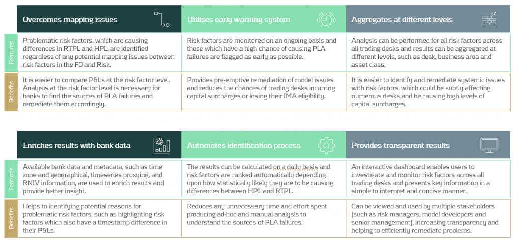
Zanders’ approach overcomes the above issues by producing analytics despite any underlying mapping issues between FO and Risk P&L data. Using our algorithm, risk factors are ranked depending upon how statistically likely they are to be causing differences between HPL and RTPL. Our metric, known as risk factor ‘alpha’, can be tracked on an ongoing basis, helping banks to remediate underlying issues with risk factors before potential PLA failures.
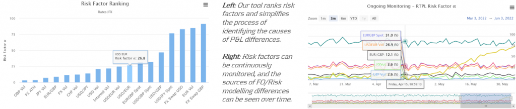
Zanders’ P&L attribution solution has been implemented at a Tier-1 bank, providing the necessary infrastructure to identify problematic risk factors and improve PLA desk statuses. The solution provided multiple benefits to increase efficiency and transparency of workstreams at the bank.
Conclusion
As it is a new regulatory requirement, passing the PLA test has been a key concern for many banks. Although the test itself is not considerably difficult to implement, identifying why a desk may be failing can be complicated. In this article, we present a PLA tool which has already been successfully implemented at one of our large clients. By helping banks to identify the underlying risk factors which are causing desks to fail, remediation becomes much more efficient. Efficient remediation of desks which are failing PLA, in turn, reduces the amount of capital charges which banks may incur.
CEO Statement: Why Our Purpose Matters

CEO Laurens Tijdhof explains the origins and importance of the Zanders group’s purpose.
The Zanders purpose
Our purpose is to deliver financial performance when it counts, to propel organizations, economies, and the world forward.
Recently, we have embarked on a process to align more effectively what we do with the changing needs of our clients in unprecedented times. A central pillar of this exercise was an in-depth dialogue with our clients and business partners around the world. These conversations confirmed that Zanders is trusted to translate our deep financial consultancy knowledge into solutions that answer the biggest and most complex problems faced by the world's most dynamic organizations. Our goal is to help these organizations withstand the current macroeconomic challenges and help them emerge stronger. Our purpose is grounded on the above.
"Zanders is trusted to translate our deep financial consultancy knowledge into solutions, answering the biggest and most complex problems faced by the world's most dynamic organizations."
Laurens Tijdhof

Our purpose is a reflection of what we do now, but it's also about what we need to do in the future.
It reflects our ongoing ambition - it's a statement of intent - that we should and will do more to affect positive change for both the shareholders of today and the stakeholders of tomorrow. We don't see that kind of ambition as ambitious; we see it as necessary.
The Zanders’ purpose is about the future. But it's also about where we find ourselves right now - a pandemic, high inflation and rising interest rates. And of course, climate change. At this year's Davos meeting, the latest Disruption Index was released showing how macroeconomic volatility has increased 200% since 2017, compared to just 4% between 2011 and 2016.
So, you have geopolitical volatility and financial uncertainty fused with a shifting landscape of regulation, digitalization, and sustainability. All of this is happening at once, and all of it is happening at speed.
The current macro environment has resulted in cost pressures and the need to discover new sources of value and growth. This requires an agile and adaptive approach. At Zanders, we combine a wealth of expertise with cutting-edge models and technologies to help our clients uncover hidden risks and capitalize on unseen opportunities.
However, it can't be solely about driving performance during stable times. This has limited value these days. It must be about delivering performance despite macroeconomic headwinds.
For over 30 years, through the bears, the bulls, and black swans, organizations have trusted Zanders to deliver financial performance when it matters most. We've earned the trust of CFOs, CROs, corporate treasurers and risk managers by delivering results that matter, whether it's capital structures, profitability, reputation or the environment. Our promise of "performance when it counts" isn't just a catchphrase, but a way to help clients drive their organizations, economies, and the world forward.
"For over 30 years, through the bears, the bulls, and black swans, financial guardians have trusted Zanders to deliver financial performance when it matters most."
Laurens Tijdhof
What "performance when it counts" means.
Navigating the current changing financial environment is easier when you've been through past storms. At Zanders, our global team has experts who have seen multiple economic cycles. For instance, the current inflationary environment echoes the Great Inflation of the 1970s. The last 12 months may also go down in history as another "perfect storm," much like the global financial crisis of 2008. Our organization's ability to help business and government leaders prepare for what's next comes from a deep understanding of past economic events. This is a key aspect of delivering performance when it counts.
The other side of that coin is understanding what's coming over the horizon. Performance when it counts means saying to clients, "Have you considered these topics?" or "Are you prepared to limit the downside or optimize the upside when it comes to the changing payments landscape, AI, Blockchain, or ESG?" Waiting for things to happen is not advisable since they happen to you, rather than to your advantage. Performance when it counts drives us to provide answers when clients need them, even if they didn't know they needed them. This is what our relationships are about. Our expertise may lie in treasury and risk, but our role is that of a financial performance partner to our clients.
How technology factors into delivering performance when it counts.
Technology plays a critical role in both Treasury and Risk. Real-time Treasury used to be an objective, but it's now an imperative. Global businesses operate around the clock, and even those in a single market have customers who demand a 24/7/365 experience. We help transform our clients to create digitized, data-driven treasury functions that power strategy and value in this real-time global economy.
On the risk management front, technology has a two-fold power to drive performance. We use risk models to mitigate risk effectively, but we also innovate with new applications and technologies. This allows us to repurpose risk models to identify new opportunities within a bank's book of business.
We can also leverage intelligent automation to perform processes at a fraction of the cost, speed, and with zero errors. In today's digital world, this combination of next generation thinking, and technology is a key driver of our ability to deliver performance in new and exciting ways.
"It’s a digital world. This combination of next generation of thinking and next generation of technologies is absolutely a key driver of our ability to deliver performance when it counts in new and exciting ways."
Laurens Tijdhof
How our purpose shapes Zanders as a business.
In closing, our purpose is what drives each of us day in and day out, and it's critical because there has never been more at stake. The volume of data, velocity of change, and market volatility are disrupting business models. Our role is to help clients translate unprecedented change into sustainable value, and our purpose acts as our North Star in this journey.
Moreover, our purpose will shape the future of our business by attracting the best talent from around the world and motivating them to bring their best to work for our clients every day.
"Our role is to help our clients translate unprecedented change into sustainable value, and our purpose acts as our North Star in this journey."
Laurens Tijdhof
VaR Backtesting in Turbulent Market Conditions: Enhancing the Historical Simulation Model with Volatility Scaling

At the end of July, the European Banking Authority (EBA) released the results on the latest installment of the EU-wide stress test that is performed every two years.
Challenges with VaR models in a turbulent market
With recent periods of market stress, including COVID-19 and the Russia-Ukraine conflict, banks are finding their VaR models under strain. A failure to adhere to VaR backtesting requirements can lead to pressure on balance sheets through higher capital requirements and interventions from the regulator.
VaR backtesting
VaR is integral to the capital requirements calculation and in ensuring a sufficient capital buffer to cover losses from adverse market conditions. The accuracy of VaR models is therefore tested stringently with VaR backtesting, comparing the model VaR to the observed hypothetical P&Ls. A VaR model with poor backtesting performance is penalised with the application of a capital multiplier, ensuring a conservative capital charge. The capital multiplier increases with the number of exceptions during the preceding 250 business days, as described in Table 1 below.

Table 1: Capital multipliers based on the number of backtesting exceptions.
The capital multiplier is applied to both the VaR and stressed VaR, as shown in equation 1 below, which can result in a significant impact on the market risk capital requirement when failures in VaR backtesting occur.


Pro-cyclicality of the backtesting framework
A known issue of VaR backtesting is pro-cyclicality in market risk. This problem was underscored at the beginning of the COVID-19 outbreak when multiple banks registered several VaR backtesting exceptions. This had a double impact on market risk capital requirements, with higher capital multipliers and an increase in VaR from higher market volatility. Consequently, regulators intervened to remove additional pressure on banks’ capital positions that would only exacerbate market volatility. The Federal Reserve excluded all backtesting exceptions between 6th – 27th March 2020, while the PRA allowed a proportional reduction in risks-not-in-VaR (RNIV) capital charge to offset the VaR increase. More recent market volatility however has not been excluded, putting pressure on banks’ VaR models during backtesting.
Historical simulation VaR model challenges
Banks typically use a historical simulation approach (HS VaR) for modelling VaR, due to its computational simplicity, non-normality assumption of returns and enhanced interpretability. Despite these advantages, the HS VaR model can be slow to react to changing markets conditions and can be limited by the scenario breadth. This means that the HS VaR model can fail to adequately cover risk from black swan events or rapid shifts in market regimes. These issues were highlighted by recent market events, including COVID-19, the Russia-Ukraine conflict, and the global surge in inflation in 2022. Due to this, many banks are looking at enriching their VaR models to better model dramatic changes in the market.
Enriching HS VaR models
Alternative VaR modelling approaches can be used to enrich HS VaR models, improving their response to changes in market volatility. Volatility scaling is a computationally efficient methodology which can resolve many of the shortcomings of HS VaR model, reducing backtesting failures.
Enhancing HS VaR with volatility scaling
The Volatility Scaling methodology is an extension of the HS VaR model that addresses the issue of inertia to market moves. Volatility scaling adjusts the returns for each time t by the volatility ratio σT/σt, where σt is the return volatility at time t and σT is the return volatility at the VaR calculation date. Volatility is calculated using a 30-day window, which more rapidly reacts to market moves than a typical 1Y VaR window, as illustrated in Figure 1. As the cost of underestimation is higher than overestimating VaR, a lower bound to the volatility ratio of 1 is applied. Volatility scaling is simple to implement and can enrich existing models with minimal additional computational overhead.
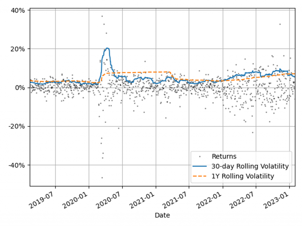
Figure 1: The 30-day and 1Y rolling volatilities of the 1-day scaled diversified portfolio returns. This illustrates recent market stresses, with short regions of extreme volatility (COVID-19) and longer systemic trends (Russia-Ukraine conflict and inflation).
Comparison with alternative VaR models
To benchmark the Volatility Scaling approach, we compare the VaR performance with the HS and the GARCH(1,1) parametric VaR models. The GARCH(1,1) model is configured for daily data and parameter calibration to increase sensitivity to market volatility. All models use the 99th percentile 1-day VaR scaled by a square root of 10. The effective calibration time horizon is one year, approximated by a VaR window of 260 business days. A one-week lag is included to account for operational issues that banks may have to load the most up-to-date market data into their risk models.
VaR benchmarking portfolios
To benchmark the VaR Models, their performance is evaluated on several portfolios that are sensitive to the equity, rates and credit asset classes. These portfolios include sensitivities to: S&P 500 (Equity), US Treasury Bonds (Treasury), USD Investment Grade Corporate Bonds (IG Bonds) and a diversified portfolio of all three asset classes (Diversified). This provides a measure of the VaR model performance for both diversified and a range of concentrated portfolios. The performance of the VaR models is measured on these portfolios in both periods of stability and periods of extreme market volatility. This test period includes COVID-19, the Russia-Ukraine conflict and the recent high inflationary period.
VaR model benchmarking
The performance of the models is evaluated with VaR backtesting. The results show that the volatility scaling provides significantly improved performance over both the HS and GARCH VaR models, providing a faster response to markets moves and a lower instance of VaR exceptions.
Model benchmarking with VaR backtesting
A key metric for measuring the performance of VaR models is a comparison of the frequency of VaR exceptions with the limits set by the Basel Committee’s Traffic Light Test (TLT). Excessive exceptions will incur an increased capital multiplier for an Amber result (5 – 9 exceptions) and an intervention from the regulator in the case of a Red result (ten or more exceptions). Exceptions often indicate a slow reaction to market moves or a lack of accuracy in modelling risk.
VaR measure coverage
The coverage and adaptability of the VaR models can be observed from the comparison of the realised returns and VaR time series shown in Figure 2. This shows that although the GARCH model is faster to react to market changes than HS VaR, it underestimates the tail risk in stable markets, resulting in a higher instance of exceptions. Volatility scaling retains the conservatism of the HS VaR model whilst improving its reactivity to turbulent market conditions. This results in a significant reduction in exceptions throughout 2022.
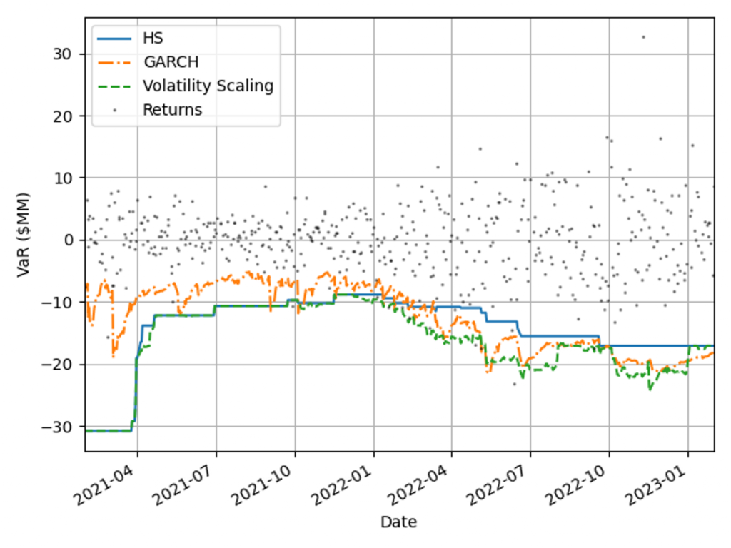
Figure 2: Comparison of realised returns with the model VaR measures for a diversified portfolio.
VaR backtesting results
The VaR model performance is illustrated by the percentage of backtest days with Red, Amber and Green TLT results in Figure 3. Over this period HS VaR shows a reasonable coverage of the hypothetical P&Ls, however there are instances of Red results due to the failure to adapt to changes in market conditions. The GARCH model shows a significant reduction in performance, with 32% of test dates falling in the Red zone as a consequence of VaR underestimation in calm markets. The adaptability of volatility scaling ensures it can adequately cover the tail risk, increasing the percentage of Green TLT results and completely eliminating Red results. In this benchmarking scenario, only volatility scaling would pass regulatory scrutiny, with HS VaR and GARCH being classified as flawed models, requiring remediation plans.
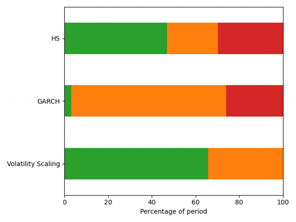
Figure 3: Percentage of days with a Red, Amber and Green Traffic Light Test result for a diversified portfolio over the window 29/01/21 - 31/01/23.
VaR model capital requirements
Capital requirements are an important determinant in banks’ ability to act as market intermediaries. The volatility scaling method can be used to increase the HS capital deployment efficiency without compromising VaR backtesting results.
Capital requirements minimisation
A robust VaR model produces risk measures that ensure an ample capital buffer to absorb portfolio losses. When selecting between robust VaR models, the preferred approach generates a smaller capital charge throughout the market cycle. Figure 4 shows capital requirements for the VaR models for a diversified portfolio calculated using Equation 1, with 𝐴𝑑𝑑𝑜𝑛𝑠 set to zero. Volatility scaling outperforms both models during extreme market volatility (the Russia-Ukraine conflict) and the HS model in period of stability (2021) as a result of setting the lower scaling constraint. The GARCH model underestimates capital requirements in 2021, which would have forced a bank to move to a standardised approach.
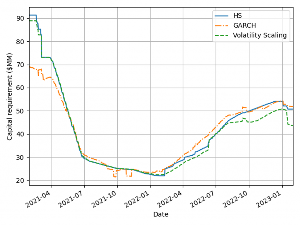
Figure 4: Capital charge for the VaR models measured on a diversified portfolio over the window 29/01/21 - 31/01/23.
Capital management efficiency
Pro-cyclicality of capital requirements is a common concern among regulators and practitioners. More stable requirements can improve banks’ capital management and planning. To measure models’ pro-cyclicality and efficiency, average capital charges and capital volatilities are compared for three concentrated asset class portfolios and a diversified market portfolio, as shown in Table 2. Volatility scaling results are better than the HS model across all portfolios, leading to lower capital charges, volatility and more efficient capital allocation. The GARCH model tends to underestimate high volatility and overestimate low volatility, as seen by the behaviour for the lowest volatility portfolio (Treasury).
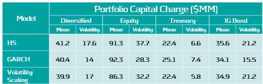
Table 2: Average capital requirement and capital volatility for each VaR model across a range of portfolios during the test period, 29/01/21 - 31/01/23.
Conclusions on VaR backtesting
Recent periods of market stress highlighted the need to challenge banks’ existing VaR models. Volatility scaling is an efficient method to enrich existing VaR methodologies, making them robust across a range of portfolios and volatility regimes.
VaR backtesting in a volatile market
Ensuring VaR models conform to VaR backtesting will be challenging with the recent period of stressed market conditions and rapid changes in market volatility. Banks will need to ensure that their VaR models are responsive to volatility clustering and tail events or enhance their existing methodology to cope. Failure to do so will result in additional overheads, with increased capital charges and excessive exceptions that can lead to additional regulatory scrutiny.
Enriching VaR Models with volatility scaling
Volatility scaling provides a simple extension of HS VaR that is robust and responsive to changes in market volatility. The model shows improved backtesting performance over both the HS and parametric (GARCH) VaR models. It is also robust for highly concentrated equity, treasury and bond portfolios, as seen in Table 3. Volatility scaling dampens pro-cyclicality of HS capital requirements, ensuring more efficient capital planning. The additional computational overhead is minimal and the implementation to enrich existing models is simple. Performance can be further improved with the use of hybrid models which incorporate volatility scaling approaches. These can utilise outlier detection to increase conservatism dynamically with increasingly volatile market conditions.
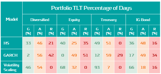
Table 3: Percentage of Green, Amber and Red traffic Lights test results for each VaR model across a range of portfolios for dates in the range: 13/02/19 - 31/01/23.
Zanders recommends
Banks should invest in making their VaR models more robust and reactive to ensure capital costs and the probability of exceptions are minimised. VaR models enriched with a volatility scaling approach should be considered among a suite of models to challenge existing VaR model methodologies. Methods similar to volatility scaling can also be applied to parametric and semi-parametric models. Outlier detection models can be used to identify changes in market regime as either feeder models or early warning signals for risk managers
Regulatory timelines ESG Risk Management

CEO Laurens Tijdhof explains the origins and importance of the Zanders group’s purpose.
In the below overview, we present an overview of the main ESG-related publications from the European Commission (EC), the European Central Bank (ECB), and the European Banking Authority (EBA).
This is complemented by the most important timelines that are stipulated in these regulations and guidelines. Additional regulations and guidelines that are expected for the next couple of years are also highlighted.
If you want to discuss any of them, don’t hesitate to reach out to our subject matter experts.
The ESG data challenge

At the end of July, the European Banking Authority (EBA) released the results on the latest installment of the EU-wide stress test that is performed every two years.
But to seize the opportunities ESG must become an integrated part of a bank’s strategy, risk management and disclosure regimes. High-quality data is instrumental to identify and measure ESG risks, but it can be lacking. FIs need to improve their internal data and use of external private and public vendors like Moody’s or the IMF, while developing a framework that plugs any data gaps.
The lack of appropriate ESG data is considered one of the main challenges for many FIs, but proxies, such as using a building’s energy rating to work out its carbon emissions, can be used.
FIs need climate change-related data that isn’t always available if you don’t know where to look. This article will give you an overview of the most relevant data vendors and provide suggestions on how to treat missing data gaps in order to get a comprehensive ESG framework for the green future where carbon measurement, assessment, reporting and trading will be vital
The data challenge
In May 2021, the Network for Greening the Financial System (NGFS) published a ‘Progress report on bridging data gaps’. In this report, the NGFS writes that meeting climate-related data needs is a challenge that can be described along the following three dimensions:
- data availability,
- reliability,
- & comparability.
A further breakdown of the challenges related to these dimensions can be found in Figure 1.
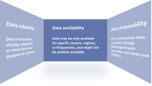
Figure 1: The dimensions of the climate-related data challenge.
Source: Graphic adapted by Zanders from a NGFS report entitled: ‘Progress report on bridging data gaps’ (2021).
Key financial metrics
The NGFS writes that a mix of policy interventions is necessary to ensure climate-related data is based on three building blocks:
- Common and consistent global disclosure standards.
- A minimally accepted global taxonomy.
- Consistent metrics, labels, and methodological standards.
EU Taxonomy, CSRD & EBA’s 3 ESG risk disclosure standards
Several initiatives have started to ignite these needed policy interventions. For example, the EU Taxonomy, introduced by the European Commission (EC), is a classification system for environmentally sustainable activities. In addition, the recently approved Corporate Sustainability Reporting Directive (CSRD) provides ESG reporting rules for large listed and non-listed companies in the EU, including several FIs. The aim of the CSRD is to prevent greenwashing and to provide the basis for global sustainability reporting standards. Another example of a disclosure standard is the binding standards on Pillar 3 disclosures on ESG risks developed by the European Banking Authority (EBA).
Even though policy, law and regulation makers have a big part to play in the data challenge, there are also steps that individual institutions could and should take to improve their own ESG data gaps. Regulatory bodies such as the EBA and the European Central Bank (ECB) have shared their expectations and recommendations on the management of ESG data with FIs.
To illustrate, the EBA recommends FIs “[identify] the gaps they are facing in terms of data and methodologies and take remedial action” and the ECB expects institutions to “assess their data needs in order to inform their strategy-setting and risk management, to identify the gaps compared with current data and to devise a plan to overcome these gaps and tackle any insufficiencies”
Collecting data
Collecting ESG data is a challenging exercise. A distinction can be made between collecting data for large market cap companies, and small cap companies and retail clients. Although large cap companies tend to be more transparent, the data often is dispersed over multiple reports – for example, corporate sustainability reports, annual reports, emissions disclosures, company websites, and so on.
For small cap companies and retail clients, the data is more difficult to acquire. Data that is not publicly available could be gathered bilaterally from clients. For example, one European bank has developed an annual client questionnaire to collect data from its clients.
Gathering data from various reports or bilaterally from clients might not always be the best option, however, because it is time consuming or because the data is not available, reliable, or comparable. Two alternatives are:
- Use tools to collect the data. For example, using open-source tooling from the Two Degrees Investing Initiative (2DII) to calculate Paris Agreement Capital Transition Assessment (PACTA) portfolio alignment.
- Collect data from other external data sources, such as S&P Global.
This could be forward-looking external data on macro-economic expectations, international climate scenarios, financial market data or sectoral climate developments. Below we discuss some sources for external ESG and climate change-related data.
External data
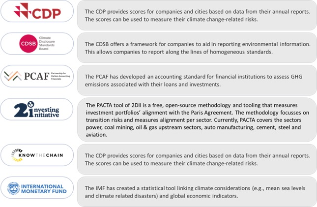
Some of Zanders’ clients resort to vendor solutions for acquiring their ESG data. The most commonly observed solutions, in random order, are:
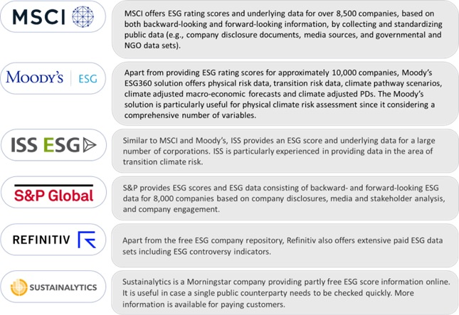
All the solutions above provide an aid to determine if climate related performance data is lacking, or can assist in reporting comparable and reliable data. They all apply a similar process of collecting the data and determining ESG scores, which is illustrated in Figure 2.
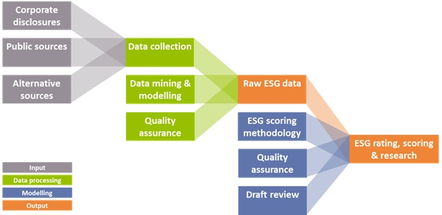
Figure 2: Data collection process for ESG data solutions (Source: Zanders).
Additionally, public and non-commercial data and solution providers are available, such as:
Missing data
Given the data challenges, it is nearly impossible to create a complete data set. Until that is possible, there are several (temporary) methods to deal with missing data:
- Find a comparable loan, asset, or company for which the required data is available.
- Distribute sector data based on market share of individual companies. For example, assign 10% of the estimated emission of sector X to company Y based on its market share of 10%.
- Find a proxy, comparable or second-best metric. For example, by taking the energy label as a proxy for CO2 emission related to properties, or by excluding scope 3 emissions and focusing on scope 1 and 2 emissions.
- Change the granularity level. For example, by gathering data on sector level rather than on individual positions.
- Fill in the gaps with statistical or machine learning techniques.
Conclusion
The increased attention to integrating ESG risks into existing risk frameworks has led to a need for FIs to collect and disclose meaningful data on ESG factors. However, there is still a lack of data availability, reliability, and comparability.
Several regulatory and political efforts are ongoing to tackle this data challenge, such as the EU taxonomy. More policy interventions, however, are required. Examples are additional mandatory disclosure requirements, an audit and validation framework for ESG data, and social and governance taxonomies that classify economic activities that contribute to social and governance goals.
In the meantime, FIs have to find ways to produce meaningful insights and comply with regulatory requirements related to ESG risks. Zanders has experienced that there is no one-size-fits-all solution for defining, selecting, implementing, and disclosing relevant data and metrics. It is dependent on the composition of the asset and loan portfolio, the use of the data, and the data that is (already) available. Regardless of how the lack of data is solved, it is important that FIs are transparent about their choices and methodologies, and that the related metrics and scorings are explainable and intuitive.
Sources:
https://www.ngfs.net/sites/default/files/medias/documents/progress_report_on_bridging_data_gaps.pdf
https://ec.europa.eu/info/business-economy-euro/banking-and-finance/sustainable-finance/eu-taxonomy-sustainable-activities_en
https://www.europarl.europa.eu/news/en/press-room/20220620IPR33413/new-social-and-environmental-reporting-rules-for-large-companies
https://zandersgroup.com/en/insights/blog/ebas-binding-standards-on-pillar-3-disclosures-on-esg-risks
https://www.eba.europa.eu/sites/default/documents/files/document_library/Publications/Reports/2021/1015656/EBA%20Report%20on%20ESG%20risks%20management%20and%20supervision.pdf
https://www.bankingsupervision.europa.eu/ecb/pub/pdf/ssm.202011finalguideonclimate-relatedandenvironmentalrisks~58213f6564.en.pdf
https://2degrees-investing.org/resource/pacta/
Integrating ESG risks into a bank’s credit risk framework

CEO Laurens Tijdhof explains the origins and importance of the Zanders group’s purpose.
The last three to four years have seen a rapid increase in the number of publications and guidance from regulators and industry bodies. Environmental risk is currently receiving the most attention, triggered by the alarming reports from the Intergovernmental Panel on Climate Change (IPCC). These reports show that it is a formidable, global challenge to shift to a sustainable economy in order to reduce environmental impact.
Zanders’ view
Zanders believes that banks have an important role to play in this transition. Banks can provide financing to corporates and households to help them mitigate or adapt to climate change, and they can support the development of new products such as sustainability-linked derivatives. At the same time, banks need to integrate ESG risk factors into their existing risk processes to prepare for the new risks that may arise in the future. Banks and regulators so far have mostly focused on credit risk.
We believe that the nature and materiality of ESG risks for the bank and its counterparties should be fully understood, before making appropriate adjustments to risk models such as rating, pricing, and capital models. This assessment allows ESG risks to be appropriately integrated into the credit risk framework. To perform this assessment, banks may consider the following four steps:
- Step 1: Identification. A bank can identify the possible transmission channels via which ESG risk factors can impact the credit risk profile of the bank. This can be through direct exposures, or indirectly via the credit risk profile of the bank’s counterparties. This can for example be done on portfolio or sector level.
- Step 2: Materiality. The materiality of the identified ESG risk factors can be assessed by assigning them scores on impact and likelihood. This process can be supported by identifying (quantitative) internal and external sources from the Network for Greening the Financial System (NGFS), governmental bodies, or ESG data providers.
- Step 3: Metrics. For the material ESG risk factors, relevant and feasible metrics may be identified. By setting limits in line with the Risk Appetite Statement (RAS) of the bank, or in line with external benchmarks (e.g., a climate science-based emission path that follows the Paris Agreement), the exposure can be managed.
- Step 4: Verification. Because of the many qualitative aspects of the aforementioned steps, it is important to verify the outcomes of the assessment with portfolio and credit risk experts.
Key insights
Prior to the roundtable, Zanders performed a survey to understand the progress that Dutch banks are marking with the integration of ESG risks into their credit risk framework, and the challenges they are facing.
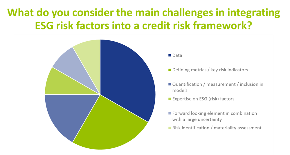
Currently, when it comes to incorporating ESG risks in the credit risk framework, banks are mainly focusing their attention on risk identification, the materiality assessment, risk metric definition and disclosures. The survey also reveals that the level of maturity with respect to ESG risk mitigation and risk limits differs significantly per bank. Nevertheless, the participating banks agreed that within one to three years, ESG risk factors are expected to be integrated in the key credit risk management processes, such as risk appetite setting, loan origination, pricing, and credit risk modeling. Data availability, defining metrics and the quantification of ESG risks were identified by banks as key challenges when integrating ESG in credit risk processes, as illustrated in the graph below.
In addition to the challenges mentioned above, discussion between participating banks revealed the following insights:
- Insight 1: Focus of ESG initiatives is on environmental factors. Most banks have started integrating environmental factors into their credit risk management processes. In contrast, efforts for integrating social and governance factors are far less advanced. Participants in the roundtable agreed that progress still has to be made in the area of data, definitions, and guidelines, before social and governance factors can be incorporated in a way that is similar to the approach for environmental factors.
- Insight 2: ESG adjustments to risk models may lead to double counting. The financial market still needs to gain more understanding to what extent ESG risk factor will manifest itself via existing risk drivers. For example, ESG factors such as energy label or flood risk may already be reflected in market prices for residential real estate. In that case, these ESG factors will automatically manifest itself via the existing LGD models and separate model adjustments for ESG may lead to double counting of ESG impact. Research so far shows mixed signals on this. For example, an analysis of housing prices by researchers from Tilburg University in 2021 has shown that there is indeed a price difference between similar houses with different energy labels. On the other hand, no unambiguous pricing differentiation was found as part of a historical house price analysis by economists from ABN AMRO in 2022 between similar houses with different flood risks. Participating banks agreed that further research and guidance from banks and the regulators is necessary on this topic.
- Insight 3: ESG factors may be incorporated in pricing. An outcome of incorporating ESG in a credit risk framework could be that price differentiation is introduced between loans that face high versus low climate risk. For example, consideration could be given to charging higher rates to corporates in polluting sectors or ones without an adequate plan to deal with the effects of climate change. Or to charge higher rates for residential mortgages with a low energy label or for the ones that are located in a flood-prone area. Participating banks agreed that in theory, price differentiation makes sense and most of them are investigating this option as a risk mitigating strategy. Nevertheless, some participants noted that, even if they would be able to perfectly quantify these risks in terms of price add-ons, they were not sure if and how (e.g., for which risk drivers and which portfolios) they would implement this. Other mitigating measures are also available, such as providing construction deposits to clients for making their homes more sustainable.
Conclusion
Most participating banks have made efforts to include ESG risk factors in their credit risk management processes. Nevertheless, many efforts are still required to comply with all regulatory expectations regarding this topic. Not only efforts by the banks themselves but also from researchers, regulators, and the financial market in general.
Zanders has already supported several banks and asset managers with the challenges related to integrating ESG risks into the risk organization. If you are interested in discussing how we can help your organization, please reach out to Sjoerd Blijlevens or Marije Wiersma.
Climate change risk

At the end of July, the European Banking Authority (EBA) released the results on the latest installment of the EU-wide stress test that is performed every two years.
The Working Group II contribution to the IPCC’s Sixth Assessment Report states that “climate change is a grave and mounting threat to our wellbeing and a healthy planet”. It is a formidable, global challenge to transition to a sustainable economy before time is running out. Banks have an important role to play in this transition. By stepping up to this role now, banks will be better prepared for the future, and reap the benefits along the way.
In the Paris Agreement (or COP21), adopted in December 2015, 196 parties agreed to limit global warming to well below 2.0°C, and preferably to no more than 1.5°C. To prevent irreversible impacts to our climate, the IPCC stresses that the increase in global temperature (relative to the pre-industrial era) needs to remain below 1.5°C. To achieve this target, a rapid and unprecedented decrease in the emission of greenhouse gasses (GHG) is required. With CO2 emissions still on the rise, as depicted in Figure 1, the challenge at hand has increased considerably in the past decade.
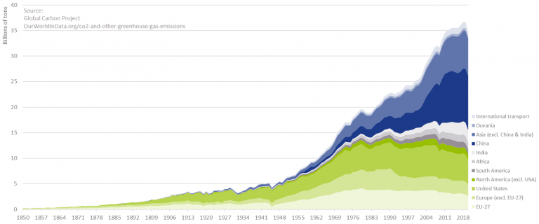
Figure 1 – Annual CO2 emissions from fossil fuels.
To further illustrate this, Figure 2 depicts for several starting years a possible pathway in CO2 reductions to ensure global warming does not exceed 2.0°C. Even under the assumption that CO2 emissions have already peaked, it becomes clear that the required speed of CO2 reductions is rapidly increasing with every year of inaction. We are a long way from limiting global warming to 2.0°C. This even holds under the assumption that all countries’ pledges to reduce GHG emissions will be achieved, as can be observed in Figure 3.
To quote the IPCC Working Group II co-chair Hans-Otto Pörtner: “Any further delay in concerted anticipatory global action on adaptation and mitigation will miss a brief and rapidly closing window of opportunity to secure a livable and sustainable future for all.”
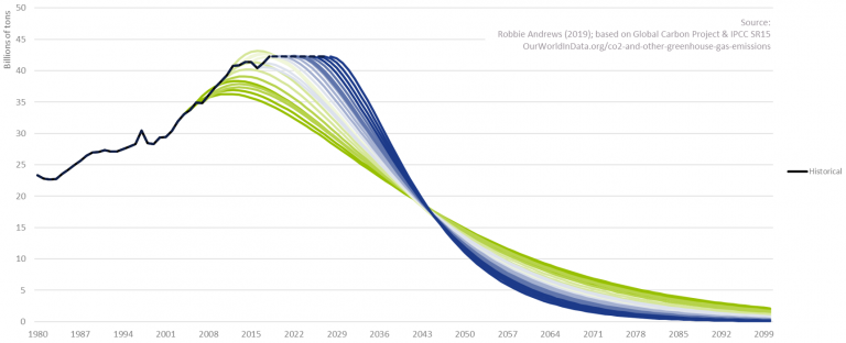
Figure 2 – CO2 reduction need to limit global warming.
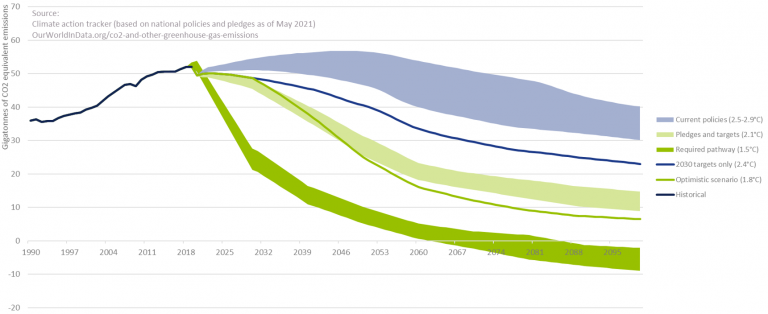
Figure 3 – Global GHG emissions and warming scenario’s.
The role of banks in the transition – and the opportunities it offers
Historically, banks have been instrumental to the proper functioning of the economy. In their role as financial intermediaries, they bring together savers and borrowers, support investment, and play an important role in facilitating payments and transactions. Now, banks have the opportunity to become instrumental to the proper functioning of the planet. By allocating their available capital to ‘green’ loans and investments at the expense of their ‘brown’ counterparts, banks can play a pivotal role in the transition to a sustainable economy. Banks are in the extraordinary position to make a fundamentally positive contribution to society. And even better, it comes with new opportunities.
The transition to a sustainable economy requires huge investments. It ranges from investments in climate change adaption to investments in GHG emission reductions: this covers for example investments in flood risk warning systems and financing a radical change in our energy mix from fossil-fuel based sources (like coal and natural gas) to clean energy sources (like solar and wind power). According to the Net Zero by 2050 Report from the International Energy Agency (IEA)2, the annual investments in the energy sector alone will increase from the current USD 2.3 trillion to USD 5.0 trillion by 2030. Hence, across sectors, the increase in annual investments could easily be USD 3.0 to 4.0 trillion. As much as 70% of this investment may need to be financed by the private sector (including banks and other financial institutions)3. To put this in perspective, the total outstanding credit to non-financial corporates currently stands at USD 86.3 trillion4. Assuming an average loan maturity of 5 years, this would translate to a 12-16% increase in loans and investments by banks on a global level. Hence, the transition to a sustainable economy will open up a large market for banks through direct investments and financing provided to corporates and households.
The transition to a sustainable economy is also triggering product development. The Climate Bonds Initiative (CBI) for example reports that the combined issuance of Environmental, Social, and Governance (ESG) bonds, sustainability-linked bonds and transition debt reached almost USD 500 billion in 2021H1, representing a 59% year-on-year growth rate. Other initiatives include the introduction of ‘green’ exchange-traded funds (ETFs) and sustainability-linked derivatives. The latter first appeared in 2019 and they provide an incentive for companies to achieve sustainable performance targets. If targets are met, a company is for example eligible for a more attractive interest coupon. Again, this is creating an interesting market for banks.
By embracing the transition, with all the opportunities that it offers, banks are also bracing themselves for the future. Banks that adopt climate change-resilient business models and integrate climate risk management into their risk frameworks will be much better positioned than banks that do not. They will be less exposed to climate-related risks, ranging from physical and transition risks to risks stemming from a reputational perspective or litigation, also justifying lower capital requirements. The early adaptors of today will be the leaders of tomorrow.
A roadmap supporting the transition
How should a bank approach this transition? As depicted in Figure 4, we identify four important steps: target setting, measurement and reporting, strategy and risk framework, and engaging with clients.
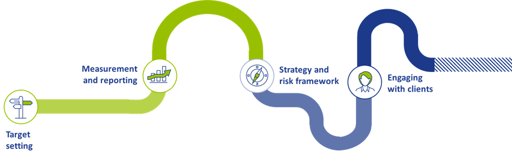
Figure 4 – The roadmap supporting the transition to a sustainable economy.
Target setting
The starting point for each transition is to set GHG emission targets in alignment with emission pathways that have been established by climate science. One important initiative that can support banks in setting these targets is the Science Based Targets initiative (SBTi). This organization supports companies to set targets in line with the goals of the Paris Agreement. Unlike many other companies, the majority of a bank’s GHG emissions are outside their direct control. They can influence, however, their so-called financed emissions, which are the GHG emissions coming from their lending and investment portfolios. The SBTi has developed a framework for banks that reflects this. It encourages banks to use the Absolute Contraction approach that requires a 2.5% (for a well-below 2.0°C target) or 4.2% (for a 1.5°C target) annual reduction in GHG emissions. A clear emission pathway guides banks in the subsequent steps of the transition process.
Measurement and reporting
With targets in place, the next important step for a bank is to determine their level of GHG emissions: both for scope 1 and 2 (the GHG emissions they control) and for scope 3 (the financed emissions). Important initiatives for the quantification of the financed emissions are the Paris Agreement Capital Transition Assessment (PACTA) and the Platform Carbon Accounting Financials (PCAF). PCAF is a Dutch initiative to deliver a global, standardized GHG accounting and reporting approach for financial institutions (building on the GHG Protocol). PACTA enables banks to measure the alignment of financial portfolios with climate scenarios.
By keeping track of the level of GHG emissions on an annual basis, banks can assess whether they are following their selected emission pathway. Reporting, in line with the recommendations of the Task Force on Climate-Related Financial Disclosures (TCFD), will contribute to a greater understanding of climate risks with their investors and other stakeholders.
Strategy and risk framework
Setting targets and measuring the current level of GHG emissions are necessary but not sufficient conditions to achieve a successful transition. Climate change risk needs to be fully integrated into a bank’s strategy and its risk framework. To assess the climate change-resilience of a bank’s strategy, a logical first step is to understand which climate change risks are material to the organization (e.g., by composing a materiality matrix). Subsequently, studying the transmission channels of these risks using scenario analysis and/or stress testing creates an understanding of what parts of the business model and lending portfolio are most exposed. This could lead to general changes in a bank’s positioning, but these risks should also be factored into the bank’s existing risk framework. Examples are the loan origination process, capital calculations, and risk reporting.
Engaging with clients
A fourth step in the game plan to successfully support the transition is for a bank to actively engage with its clients. A dialogue is required to align the bank’s GHG emission targets with those of its clients. This extends to discussing changes in the operations and/or business model of a client to align with a sustainable economy. This also may include timely announcing that certain economic activities will no longer be financed, and by financing client’s initiatives to mitigate or adapt to climate change: e.g., financing wind turbines for clients with energy- or carbon-intensive production processes (like cement or aluminium) or financing the move of production locations to less flood-prone areas.
Conclusion
Banks are uniquely positioned to play a pivotal role in the transition to a sustainable economy. The transition is already providing a wide range of opportunities for banks, from large financing needs to the introduction of green bonds and sustainability-linked derivatives. At the same time, it is of paramount importance for banks to adopt a climate change-resilient strategy and to integrate climate change risk into their risk frameworks. With our extensive track record in financial and non-financial risk management at financial institutions, Zanders stands ready to support you with this ambitious, yet rewarding challenge.
ESG risk management and Zanders
Zanders is currently supporting several clients with the identification, measurement, and management of ESG risks. For a start, we are supporting a large Dutch bank with the identification of ESG risk factors that have a material impact on the credit risk profile of its portfolio of corporate loans. The material risk factors are then integrated in the bank’s existing credit risk framework to ensure a proper management of this new risk type.
We are supporting other banking clients with the quantification of climate change risk. In one case, we are determining climate change risk-adjusted Probabilities of Default (PDs). Using expected future emissions and carbon prices based on the climate change scenarios of the Network for Greening the Financial System (NGFS), company specific shocks based on carbon prices and country specific shocks on GDP level are determined. These shocked levels are then used to determine the impact on the forecasted PDs. In another case, we are investigating the potential impact of floods and droughts on the collateral value of a portfolio of residential mortgage loans.
We also gained experience with the data challenges involved in the typical ESG project: e.g., we are supporting an asset manager with integrating and harmonizing ESG data from a range of vendors, which is underlying their internally developed ESG scores. We also support them with embedding these scores in the investment process.
With our extensive track record in financial and non-financial risk management at financial institutions in general, and our more recent ESG experience, Zanders stands ready to support you with the ambitious, yet rewarding challenge to adopt a climate change-resilient strategy and to integrate climate change risk in your existing risk frameworks.
Foot notes:
1 The IPCC Working Group II contribution: Climate Change 2022: Impacts, Adaptation and Vulnerability.
2 The IEA report, Net Zero by 2050.
3 See the Net Zero Financing roadmaps from the UN, ‘Race to Zero’ and the ‘Glasgow Financial Alliance for Net Zero’ (GFANZ).
4 Based on the statistics of the Bank for International Settlements (BIS) per 2021-Q3.
5 The Climate Bonds Initiative’s Sustainable Debt Highlights H1 2021.
EBA’s binding standards on Pillar 3 disclosures on ESG risks

CEO Laurens Tijdhof explains the origins and importance of the Zanders group’s purpose.
This publication fits nicely into the ‘horizon priority’ of the EBA1 to provide tools to banks to measure and manage ESG-related risks. In this article we present a brief overview of the way the ITS have been developed, what qualitative and quantitative disclosures are required, what timelines and transitional measures apply – and where the largest challenges arise. By requiring banks to disclose information on their exposure to ESG-related risks and the actions they take to mitigate those risks – for example by supporting their clients and counterparties in the adaptation process – the EBA wants to contribute to a transition to a more sustainable economy. The Pillar 3 disclosure requirements apply to large institutions with securities traded on a regulated market of an EU member state.
In an earlier report2, the EBA defined ESG-related risks as “the risks of any negative financial impact on the institution stemming from the current or prospective impacts of ESG factors on its counterparties or invested assets”. Hence, the focus is not on the direct impact of ESG factors on the institution, but on the indirect impact through the exposure of counterparties and invested assets to ESG-related risks. The EBA report also provides examples for typical ESG-related factors.
While the ITS have been streamlined and simplified compared to the consultation paper published in March 2021, there are plenty of challenges remaining for banks to implement these standards.
Development of the ITS
The EBA has been mandated to develop the ITS on P3 disclosures on ESG risks in Article 434a of the Capital Requirements Regulation (CRR). The EBA has opted for a sequential approach, with an initial focus on climate change-related risks. This is further narrowed down by only considering the banking book. The short maturity and fast revolving positions in the trading book are out of scope for now. The scope of the ITS will be extended to included other environmental risks (like loss of biodiversity), and social and governance risks, in later stages.
In the development of the ITS, the EBA has strived for alignment with several other regulations and initiatives on climate-related disclosures that apply to banks. The most notable ones are listed below (and in Figure 1):
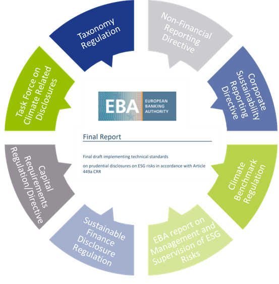
Figure 1 – Overview of related regulations and initiatives considered in the development of the ITS
- Capital Requirements Directive and Regulation (CRD and CRR): article 98(8) of the CRD3 mandated the EBA to publish the EBA report on Management and Supervision of ESG risks, which includes the split of climate change-related risks in physical and transition risks. Article 434a of the CRR4 mandated the EBA to develop the draft ITS to specify the ESG disclosure requirements described in article 449a.
- EBA report on Management and Supervision of ESG risks2: the report provides common definitions of ESG risks and contains proposals on how to include ESG risks in the risk frameworks of banks, covering its identification, assessment, and management. It also discusses the way to include ESG risks in the supervisory review process.
- Task Force on Climate-related Financial Disclosures (TCFD)5: the Financial Stability Board’s TFCD has published recommendations on climate-related disclosures. The metrics and Key Performance Indicators (KPIs) included in the ITS have been aligned with the TCFD recommendations.
- Taxonomy Regulation6: the European Union’s common classification system of environmentally sustainable economic activities is underpinning the main KPIs introduced in the ITS.
- Climate Benchmark Regulation (CBR)7: In the CBR, two types of climate benchmarks were introduced (‘EU Climate Transition’ and ‘EU Paris-aligned’ benchmarks) and ESG disclosures for all other benchmarks (excluding interest rate and currency benchmarks) were required.
- Non-Financial Reporting Directive (NFRD)8: the NFRD introduces ESG disclosure obligations for large companies, which include climate-related information.
- Corporate Sustainability Reporting Directive (CSRD)9: a proposal by the European Commission to extend the scope of the NFRD to also include all companies listed on regulated markets (except listed micro-enterprises). One of the ITS’s KPIs, the Green Asset Ratio (GAR) is directly linked to the scope of the NFRD/CSRD.
- Sustainable Finance Disclosure Regulation (SFDR)10: the SFDR lays down sustainability disclosure obligations for manufacturers of financial products and financial advisers towards end-investors. It applies to banks that provide portfolio management investment advice services.
Compared to the consultation paper for the ITS, several changes have been made to the required templates. Some templates have been combined (e.g., templates #1 and #2 from the consultation paper have been combined into template #1 of the final draft ITS) and several templates have been reorganized and trimmed down (e.g., the requirement to report exposures to top EU or top national polluters has been removed).
Quantitative disclosures
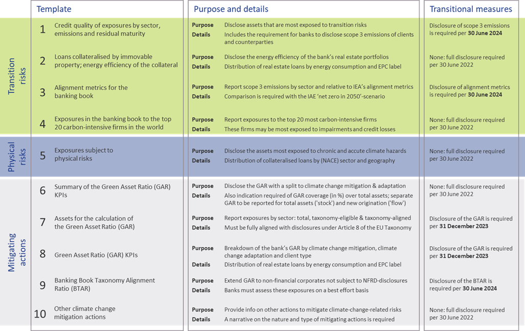
The ITS on P3 disclosure on ESG risks introduce ten templates on quantitative disclosures. These can be grouped in four templates on transition risks, one on physical risks, and five on mitigating actions:
- Transition risks
Two of the required templates are relatively straightforward. Banks need to report the energy efficiency of real estate collateral in the loan portfolio (#2) and report their aggregate exposure to the top 20 of the most carbon-intensive firms in the world (#4).
The main challenge for banks though will be in completing the other two templates:- Template #1 requires banks to disclose the gross carrying amount of loans and advances provided to non-financial corporates, classified by NACE sector codes and residual maturities. It is also required to report on the counterparties’ scope 1, 2, and 3 greenhouse gas (GHG) emissions. Reflecting the challenge in reporting on scope 3 emissions, a transitional measure is in place. Full reporting needs to be in place by June 2024. Until then, banks need to report their available estimates (if any) and explain the methodologies and data sources they intend to use.
- In the last template (#3), banks also need to report scope 3 emissions, but relate these to the alignment metrics defined by the International Energy Agency (IEA) for the ‘net zero by 2050’ scenario. For this scenario, a target for a CO2 intensity metric is defined for 2030. By calculating the distance to this target, it becomes clear how banks are progressing (over time) towards supporting a sustainable economy. A similar transitional measure applies as for template #1.
- Physical risks
In template #5, banks are required to disclose how their banking book positions are exposed to physical risks, i.e., “chronic and acute climate-related hazards”. The exposures need to be reported by residual maturity and by NACE sector codes and should reflect exposure to risks like heat waves, droughts, floods, hurricanes, and wildfires. Specialized databases need to be consulted to compile a detailed understanding of these exposures. To support their submissions, banks further need to compile a narrative that explains the methodologies they used. - Mitigating actions
The final set of templates covers quantitative information on the actions a bank takes to mitigate or adapt to climate change risks.- Templates #6-8 all relate to the GAR, which indicates what part of the bank’s banking book is aligned with the EU’s Taxonomy:
- In template #7, banks need to report the outstanding banking book exposures to different types of clients/issuers, as well as the amount of these exposures that are taxonomy-eligible (that is, to sectors included in the EU Taxonomy) and taxonomy-aligned (that is, taxonomy-eligible exposures financing activities that contribute to climate change mitigation or adaptation). Based on this information, the bank’s GAR can be determined.
- In template #8, a GAR needs to be reported for the exposures to each type of client/issuer distinguished in template #7, with a distinction between a GAR for the full outstanding stock of exposures per client/issuer type, and a GAR for newly originated (‘flow’) exposures.
- Template #6 contains a summary of the GARs from templates #7 and #8.
In these templates, the numerator of the GAR only includes exposures to non-financial corporations that are required to publish non-financial information under the NFRD. Any exposures to other corporate counterparties therefore are considered 0% Taxonomy-aligned.
- The main challenge in this group of templates is in template #9. To incentivize banks to support all of their counterparties to transition to a more sustainable business model, and to collect ESG data on these counterparties, the EBA introduces the Banking Book Taxonomy Alignment Ratio (BTAR). In this metric, the numerator does include the exposures to counterparties that are not subject to NFRD disclosure obligations. The BTAR ratios obtained from the information in template #9 therefore complement the GAR ratios obtained in templates #7 and #8.
- In the final template (#10), banks have the opportunity to include any other climate change mitigating actions that are not covered by the EU Taxonomy. They can for example report on their use of green or sustainable bonds and loans.
- Templates #6-8 all relate to the GAR, which indicates what part of the bank’s banking book is aligned with the EU’s Taxonomy:
An overview of the templates for quantitative disclosures in presented in Figure 2.
Qualitative disclosures
In the ITS on P3 disclosures on ESG risks, three tables are included for qualitative disclosures. The EBA has aligned these tables with their Report on Management and Supervision of ESG risks11. The three tables are set up for qualitative information on environmental, social, and governance risks, respectively. For each of these topics, banks need to address three aspects: on business strategy and processes, governance, and risk management. An overview of the required disclosures is presented in Figure 3.
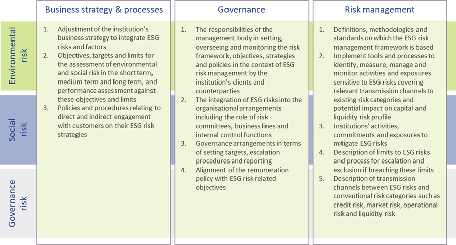
Figure 3 – Overview of qualitative ESG disclosures (based on templates & section 2.3.2 of the EBA ITS on P3 disclosures on ESG risks)
Timelines and transitional measures
The ITS on P3 disclosure on ESG risks become effective per 30 June 2022 for large institutions that have securities traded on a regulated market of an EU member state. A semi-annual disclosure is required, but the first disclosure is annual. Consequently, based on 31 December 2022 data, the first reporting will take place in the first quarter of 2023.
The EBA has introduced a number of transitional measures. These can be summarized as follows:
- The reporting of information on the GAR is only required as of 31 December 2023.
- The reporting of information on the BTAR, the bank’s financed scope 3 emissions, and the alignment metrics is only required as of June 2024.
The EBA has further indicated in the ITS that they will conduct a review of the ITS’s requirements during 2024. They may then also extend the ITS with other environmental risks (other than the climate change-related risks in the current version). The EU Taxonomy is expected to cover a broader range of environmental risks by the end of 2022. Sometime after 2024, it is expected that the EBA will further extend the ITS by including disclosure requirements on social and governance risks.
An overview of the main timelines and transitional measures is presented in Figure 4.
Figure 4 – Overview of the main timelines and transitional measures for the ESG disclosures
Conclusion
Society, and consequently banks too, are increasingly facing risks stemming from changes in our climate. In recent years, supervisory authorities have stepped up by introducing more and more guidance and regulation to create transparency about climate change risk, and more broadly ESG risks. The publication of the ITS on P3 disclosures on ESG risks by the EBA marks an important milestone. It offers banks the opportunity to disseminate a constructive and positive role in the transition to a sustainable economy.
Nonetheless, implementing the disclosure requirements will be a challenge. Developing detailed assessments of the physical risks to which their asset portfolio is exposed and to estimate the scope 3 emissions of their clients and counterparties (‘financed emissions’) will not be straightforward. For their largest counterparties, banks will be able to profit from the NFRD disclosure obligations, but especially in Europe a bank’s portfolio typically has many exposures to small- and medium-sized enterprises. Meeting the disclosure requirements introduced by the EBA will require timely and intensive discussions with a substantial part of the bank’s counterparties.
Banks also need to provide detailed information on how ESG risks are reflected in the bank’s strategy and governance and incorporated in the risk management framework. With our extensive knowledge on market risk, credit risk, liquidity risk, and business risk, Zanders is well equipped to support banks with integrating the identification, measurement, and management of climate change-related risks into existing risk frameworks. For more information, please contact Pieter Klaassen or Sjoerd Blijlevens via +31 88 991 02 00.
References
- See the EBA 2022 Work Programme.
- The EBA’s Report on Management and Supervision of ESG risks for credit institutions and investment firms, published in June 2021.
- See the EBA’s interactive Single Rulebook.
- See Regulation (EU) 2019/876.
- See the TCFD’s Final Report on Recommendations of the Task Force on Climate-related Financial Disclosures published in June 2017.
- See the EBA’s response to EC Call for Advice on Article 8 Taxonomy Regulation.
- See Regulation (EU) 2019/2089.
- See Directive 2014/95/EU.
- See the European Commission’s Proposal for a Corporate Sustainability Reporting Directive.
- See Regulation (EU) 2019/2088.
- The EBA report can be found here.


