
With IFRS 18 introducing fundamental changes to FX reporting, treasuries must act now to prepare for the 2027 compliance deadline.
IFRS 18 introduces significant changes to FX classification and reporting requirements by January 2027. Despite that this adoption date still feels quite far away, there is quite some time required in order to be compliant. Treasury Management Systems and ERP platforms must be updated to ensure compliance with new operating, investing, and financing categorizations. Introduced by the International Accounting Standards Board (IASB) in April 2024, IFRS 18 is required to be implemented by January 2027 at the latest. The new standard addresses how companies classify foreign exchange (FX) gains and losses, particularly affecting treasury operations.
In the past, for simplicity and pragmatic reasons, many organizations reported all FX results as part of operating income. Under IFRS 18 however, guidance on the treatment of these FX results is more explicit and must now be categorized into three groups: operating, investing, and financing dependent on the nature of the underlying exposure.
While this is a simple requirement conceptually, certain challenges may exist in creating a holistic transparent view on the FX impacts, particularly when considering the treatment of FX derivatives. This shift means that businesses must reassess their accounting practices and treasury and hedging strategies to ensure compliance.
Key Changes Under IFRS 18:The primary change in IFRS 18 is the requirement to classify FX gains and losses based on their source:
- Operating: FX results from accounts payable (AP) and accounts receivable (AR) transactions fall into this category.
- Investing: FX fluctuations linked to investments are recorded here.
- Financing: FX changes related to loans and borrowings belong in this section.
Key Date: Full implementation required by January 2027
The P&L impact from FX derivatives should also be considered in these changes, where the selection of P&L category is determined based on the nature of the exposure. IFRS 18 does allow for the P&L classification from FX derivatives to be entirely posted as Operating in the case where it is not practical to uniquely identify the nature of the underlying exposure.
This may be a common occurrence, specifically in the example of Balance Sheet FX hedging, where it is not common to hedge the individual elements of the balance sheet separately. While posting to Operating for derivatives is easier to achieve, it would create inconsistencies in categorization between the FX result from hedging, and the FX result from source.
The goal of IFRS 18 is to create clearer and more comparable financial statements across different businesses, therefore the treatment of FX results from hedging activities should be carefully considered.
Treasury’s Role in the Transition
The treasury department will play a crucial role in implementing IFRS 18. While the new classification rules are straightforward, their practical application requires an in-depth review of the drivers of FX exposure and the applied hedging strategies. Determining which department takes primary responsibility for IFRS 18 implementation can be challenging. The cross-functional nature of the project requires clear ownership and accountability structures to ensure successful implementation. This coordination challenge makes a strong case for external advisory support to facilitate collaboration between treasury, finance, accounting, and IT teams.
One major challenge of IFRS 18 is the potential mismatch between FX hedging strategies and accounting classifications. Traditionally, companies have managed FX risk through balance sheet hedging, using a single FX deal to cover multiple exposures. However, with the new classification rules, companies may need to adjust their hedging approach to ensure that hedge results align with the appropriate classification.
For example, if a company hedges a foreign currency loan, and the loan’s FX impact is now categorized under financing, the FX gain or loss from the hedge should also be classified under financing. If it remains under operating income, the company may see artificial volatility in financial statements, which could misrepresent its risk management effectiveness.
Operational and Systemic Adjustments
Beyond policy updates, IFRS 18 requires changes to Treasury Management Systems (TMS) and Enterprise Resource Planning (ERP) systems. These systems must be configured to ensure that FX transactions are correctly classified into operating, investing, or financing categories. This may involve adding new data fields, updating existing reporting structures, or even implementing new hedging processes.
Challenges and Considerations:
Companies may face several key challenges in implementing IFRS 18:
- Instance Structure Differences: Companies must determine how to apply classification rules across different subsidiaries and business units. Classification of operating for a finance company like the Treasury center may differ from that of a regular business operation.
- Chart of Accounts Adjustments: Treasury teams must assess whether existing FX hedging strategies need to be revised.
- System Updates: IT teams must modify TMS and ERP systems to support the new classification structure.
- Cross-Department Coordination: Treasury, finance, and accounting teams must work together to ensure a smooth transition.
How Zanders Can Help
Zanders, a leading treasury advisory firm, offers support to companies transitioning to IFRS 18. Our expertise extends beyond compliance, helping organizations develop effective hedging policies, update financial systems, and align their reporting strategies. Our services include:
- Reviewing FX exposure and hedging strategies.
- Identifying and resolving classification challenges.
- Developing a step-by-step plan for IFRS 18 compliance.
- Assisting with system updates and configuration changes in TMS and ERP platforms.
By addressing IFRS 18 proactively, treasury teams can not only comply with the new standard but also enhance their overall risk management approach. Zanders is committed to helping organizations navigate these changes efficiently.
Conclusion
IFRS 18 represents a significant shift in how FX gains and losses are reported and viewed through accounting principles and hedging strategies. While the standard itself is not overly complex, its impact on hedging and financial reporting requires careful planning, BI preparation, and compliance validation.
With the compliance deadline approaching in January 2027, now is the time to act. Zanders is ready to assist companies in this transition, providing both strategic guidance and practical implementation support to ensure a seamless adaptation to IFRS 18.
To find out more about IFRS 18 and key changes for treasury, please contact Jonathan Tomlinson or Mitchell Ponder.

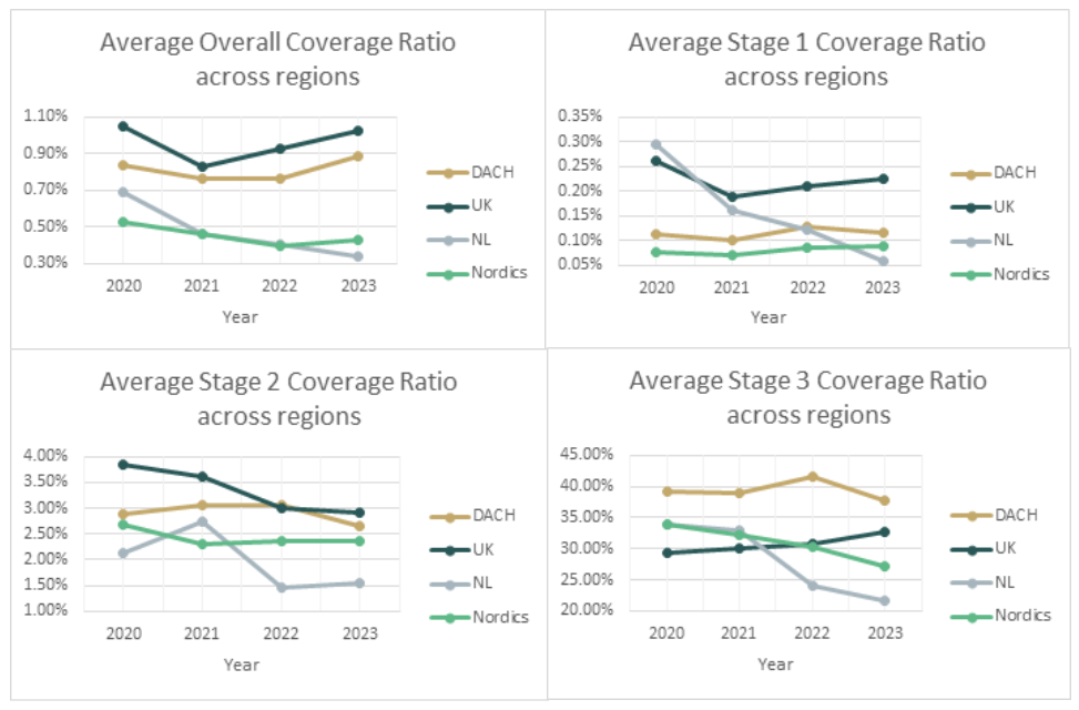
Zanders has conducted an annual report study for IFRS 9 results across 4 different European markets. These regions are the Nordics, the Netherlands, DACH and the UK.
First, these regions were analyzed independently such that common trends and differences could be noted within. These results were aggregated for each region such that these regions could be compared with each other. The results show that within European regions the year-on-year trends are similar between banks, but that across these regions the trends do differ across the years. Because the systemic macroeconomic trends the last years were similar between regions (Covid-19 and the war in Ukraine ), it shows that there are significant cultural differences in how ECLs are modelled. This shows that there is a need for alignment between European regions for which Zanders can assist. Namely, we have a presence in each of these regions and are actively monitoring development in the area of IFRS 9 (also see our previous research on IFRS 9).
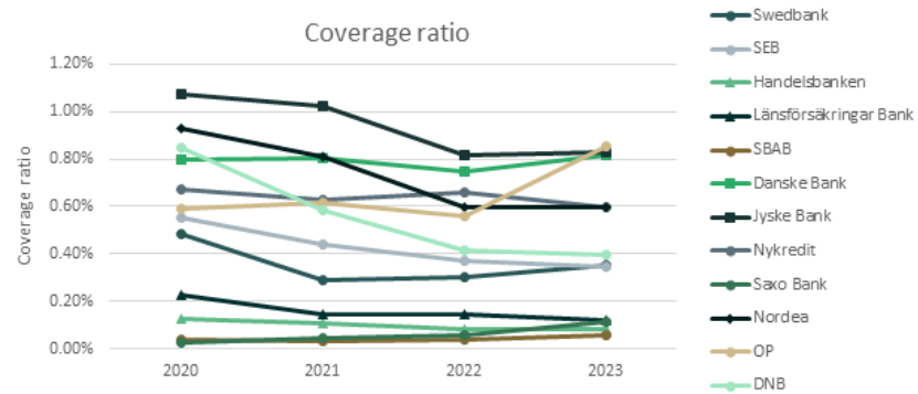
Nordics
The overall coverage ratios for most of the Danish, Swedish, Norwegian and Finnish banks1 (Nordic region) showed a slightly decreasing trend from 2020 to 2023, except for OP, which had a significant absolute increment of 0.25% to 0.86% in 2023 compared with the previous three years due to an increase in the stage 2 coverage ratio and a higher Stage 1 to 2 ratio. OP also had the highest overall coverage ratio among the sampled banks. The decreasing trend in the overall coverage ratio was primarily attributed to the decline in the Stage 3 coverage ratio.
On the other hand, the change in the Stage 1 coverage ratio was relatively stable over the years, with an absolute difference of less than 0.09% between the maximum and minimum values across the four-year period. The Stage 2 coverage ratio exhibited a similar trend across banks, except for Jyske Bank, which showed a volatile pattern, with an absolute difference of over 3% between the maximum and minimum values throughout the four years, peaking at 4.74% in 2023. In addition, the overall and the Stage 3 coverage ratios varied from 0.06% to 0.86% and 16.3% to 45.6% across banks in 2023.
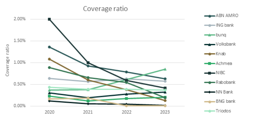
Netherlands
There was a slight decrease in the overall ECL results for the Dutch market2 over the four-year study period (also see the previous research on the Dutch market). This was primarily driven by an improved macroeconomic outlook and a further reversal of manual overlays that were applied during the COVID-19 period (e.g., ABN AMRO).
Compared with 2022, larger banks (Rabobank and ABN AMRO) showed a decrease in the overall coverage ratio with a higher weight given to the up scenario. In contrast, smaller banks tended to have a higher coverage ratio due to shifting more weight from the up scenario to the base scenario or changes in the underlying models.
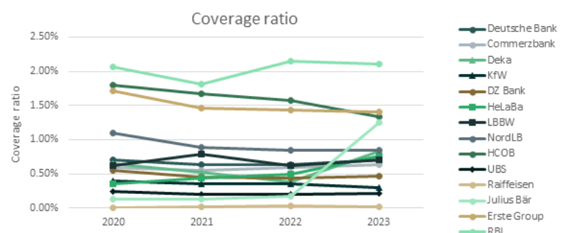
DACH
For the German, Austrian and Swiss region (DACH),3 a relatively stable trend was observed in the overall coverage ratio from 2020 to 2022, which was then countered by a sharp upward trend from 2022 to 2023. Among the banks noted, RBI stood out from its peers in reporting significantly higher overall, Stage 2 and Stage 3 coverage ratios during the study period. RBI is one of Austria's leading corporate and investment banks, operating in Central and Eastern European markets. In some Eastern European countries, Stage 2 loans remain exceptionally high, at 15 to 20 percent, leading to large overall and Stage 2 coverage ratios.
Compared to 2022, the increase in the overall coverage ratio can be attributed to higher Stage 2 coverage ratios for half of the sampled banks. Julius Bär also experienced an exceptionally high stage 3 coverage ratio of up to 93% in 2023, primarily from its Lombard loan portfolio.
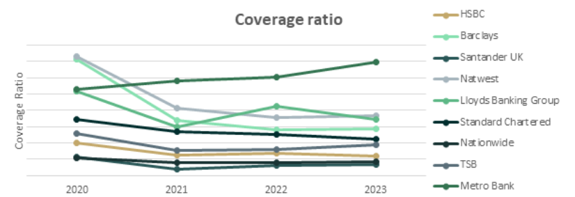
UK
During the benchmarking period from 2020 to 2023, most UK banks4 reported a decrease in the overall coverage ratio from 2020 to 2021. Then the overall coverage ratio stabilized for the remaining two years, except for one of the sampled banks, whose coverage ratio had been increasing since 2021 and recorded the second-highest overall coverage ratio in 2024 (i.e. 1.6% vs. the median of 0.8% for all sampled UK banks).
The highest coverage ratio of all years is from Monzo. As a relatively new digital bank focused on expanding, Monzo has significantly expanded its lending in recent years, with a doubling of the gross carrying amount in the latest reporting period. However, their overall coverage ratios remained high, at around 14% to 14.6% over the past two years. In the figure below (and the figures at the end of the article), Monzo has been excluded, as it individually inflated the results and rendered the other results unreadable.
Across regions
In general, all regions showed a decrease in the overall ECL coverage ratio during the initial benchmarking period, from 2020 to 2021. Compared to 2020, the coverage ratio in the most recent year has decreased, except for the DACH region, where the overall coverage ratio has reached a level comparable to that of the UK, due to a significant increase in Stage 2 numbers. The UK has the highest overall, as well as Stage 1 and Stage 2 coverage ratios, while the DACH region has the highest Stage 3 coverage ratios (i.e., the highest LGD).
In short, this shows that both the UK and DACH region demonstrate a higher overall coverage ratio, which seems to be consistent throughout all the years from 2020 onwards. Even the lowest reported average coverage ratio for the DACH region, 0.76% in 2021 is higher than the highest reported value for the Netherlands, 0.69% in 2020. As the values differ greatly between regions while the macroeconomic occurrences were similar (Covid-19, Ukraine war), it could be noted that this must be caused by significant differences in how the ECLs are modelled. And as markets are not aligned how to model ECL, it is worthwhile to further investigate how European regions can learn from each other in modeling ECL.
As Zanders has a presence in each of these regions and is in constant contact with many of the active banks in those regions, we are the best strategic partner to help improving your IFRS 9 modeling. Whether it is an independent validation of an existing model of if help is needed with the (re)development of new IFRS 9 models, we can help clients achieve the optimal accuracy with regards to their ECL estimates.
If you wish to learn more about IFRS 9 please contact Kasper Wijshoff.
Citations
- The Nordic banks that were included in the analysis were the following: Swedbank, SEB, Handelsbanken, Länsförsäkringar Bank, SBAB, Danske Bank, Jyske Bank, Nykredit, Nordea, OP, DNB. ↩︎
- The Dutch banks that were included in the analysis were the following: ABN AMRO, ING bank, bunq, Volksbank, Knab, Achmea, NIBC, Rabobank, NN Bank, BNG bank, Triodos. ↩︎
- The banks in the DACH region that were included in the analysis were the following: Deutsche Bank, Commerzbank, Deka, KfW, DZ Bank, HeLaBa, LBBW, NordLB, HCOB, UBS, Julius Bär, Erste Group, RBI. ↩︎
- The banks in the UK that were included in the analysis were the following: HSBC, Barclays, Santander UK, Natwest, Lloyds Banking Group, Standard Chartered, Monzo, Nationwide, TSB, Metro Bank, Close Brothers, Atom Bank, Revolut. ↩︎

On 18 May 2017, the International Accounting Standard Board (IASB) issued the new IFRS 17 standards. The development of these standards has been a long and thorough process with the aim of providing a single global comprehensive accounting standard for insurance contracts.
The new standards will have a significant impact on the measurement and presentation of insurance contracts in the financial statements and require significant operational changes. This article takes a closer look at the new standards, and illustrates the impact with a case study.
The standard model, as defined by IFRS 17, of measuring the value of insurance contracts is the ‘building blocks approach’. In this approach, the value of the contract is measured as the sum of the following components:
- Block 1: Sum of the future cash flows that relate directly to the fulfilment of the contractual obligations.
- Block 2: Time value of the future cash flows. The discount rates used to determine the time value reflect the characteristics of the insurance contract.
- Block 3: Risk adjustment, representing the compensation that the insurer requires for bearing the uncertainty in the amount and timing of the cash flows.
- Block 4: Contractual service margin (CSM), representing the amount available for overhead and profit on the insurance contract. The purpose of the CSM is to prevent a gain at initiation of the contract.
Risk adjustment vs risk margin
IFRS 17 does not provide full guidance on how the risk adjustment should be calculated. In theory, the compensation required by the insurer for bearing the risk of the contract would be equal to the cost of the needed capital. As most insurers within the IFRS jurisdiction capitalize based on Solvency II (SII) standards, it is likely that they will leverage on their past experience. In fact, there are many similarities between the risk adjustment and the SII risk margin.
The risk margin represents the compensation required for non-hedgeable risks by a third party that would take over the insurance liabilities. However, in practice, this is calculated using the capital models of the insurer itself. Therefore, it seems likely that the risk margin and risk adjustment will align. Differences can be expected though. For example, SII allows insurers to include operational risk in the risk margin, while this is not allowed under IFRS 17.
Liability adequacy test
Determining the impact of IFRS 17 is not straightforward: the current IFRS accounting standard leaves a lot of flexibility to determine the reserve value for insurance liabilities (one of the reasons for introducing IFRS 17). The reserve value reported under current IFRS is usually grandfathered from earlier accounting standards, such as Dutch GAAP. In general, these reserves can be defined as the present value of future benefits, where the technical interest rate and the assumptions for mortality are locked-in at pricing.
However, insurers are required to perform liability adequacy testing (LAT), where they compare the reserve values with the future cash flows calculated with ‘market consistent’ assumptions. As part of the market consistent valuation, insurers are allowed to include a compensation for bearing risk, such as the risk adjustment. Therefore, the biggest impact on the reserve value is expected from the introduction of the CSM.
The IASB has defined a hierarchy for the approach to measure the CSM at transition date. The preferred method is the ‘full retrospective application’. Under this approach, the insurer is required to measure the insurance contract as if the standard had always applied. Hence, the value of the insurance contract needs to be determined at the date of initial recognition and consecutive changes need to be determined all the way to transition date. This process is outlined in the following case study.
A case study
The impact of the new IFRS standards is analyzed for the following policy:
- The policy covers the risk that a mortgage owner deceases before the maturity of the loan. If this event occurs, the policy pays the remaining notional of the loan.
- The mortgage is issued on 31 December 2015 and has an initial notional value of € 200,000 that is amortized in 20 years. The interest percentage is set at 3 per cent.
- The policy pays an annual premium of € 150. The annual estimated costs of the policy are equal to 10 per cent of the premium.
In the case of this policy, an insurer needs to capitalize for the risk that the policy holder’s life expectancy decreases and the risk that expenses will increase (e.g. due to higher than expected inflation). We assume that the insurer applies the SII standard formula, where the total capital is the sum of the capital for the individual risk types, based on 99.5 per cent VaR approach, taking diversification into account.
The cost of capital would then be calculated as follows:
- Capital for mortality risk is based on an increase of 15 per cent of the mortality rates.
- Capital for expense risk is based on an increase of 10 per cent in expense amount combined with an increase of 1 per cent in the inflation.
- The diversification between these risk types is assumed to be 25 per cent.
- Future capital levels are assumed to be equal to the current capital levels, scaled for the decrease in outstanding policies and insurance coverage.
- The cost-of-capital rate equals 6 per cent.
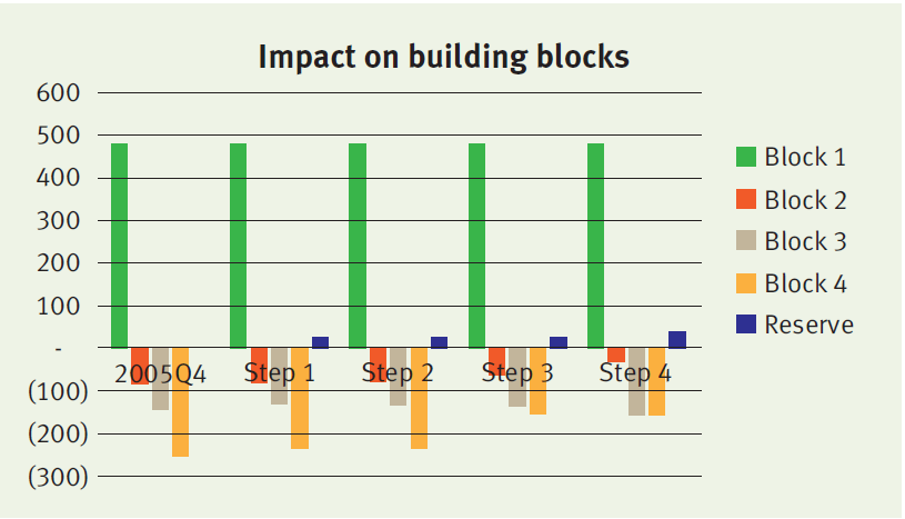
At initiation (i.e. 2015 Q4), the value of the contract under the new standards equals the sum of:
- Block 1: € 482
- Block 2: minus € 81
- Block 3: minus € 147
- Block 4: minus € 254
Consecutive changes
The insurer will measure the sum of blocks 1, 2 and 3 (which we refer to as the fulfilment cash flows) and the remaining amount of the CSM at each reporting date. The amounts typically change over time, in particular when expectations about future mortality and interest rates are updated. We distinguish four different factors that will lead to a change in the building blocks:
Step 1. Time effect
Over time, both the fulfilment cash flows and the CSM are fully amortized. The amortization profile of both components can be different, leading to a difference in the reserve value.
Step 2. Realized mortality is lower than expected
In our case study, the realized mortality is about 10 per cent lower than expected. This difference is recognized in P&L, leading to a higher profit in the first year. The effect on the fulfilment cash flows and CSM is limited. Consequently, the reserve value will remain roughly the same.
Step 3. Update of mortality assumptions
Updates of the mortality assumptions affect the fulfilment cash flows, which is simultaneously recognized in the CSM. The offset between the fulfilment cash flows and the CSM will lead to a very limited impact on the reserve value. In this case study, the update of the life table results in higher expected mortality and increased future cash outflows.
Step 4. Decrease in interest rates
Updates of the interest rate curve result in a change in the fulfilment cash flows. This change is not offset in the CSM, but is recognized in the other comprehensive income. Therefore a decrease in the discount curve will result in a significant change in the insurance liability. Our case study assumes a decrease in interest rates from 2 per cent to 1 per cent. As a result, the fulfilment cash flows increase, which is immediately reflected by an increase in the reserve value.
The impact of each step on the reserve value and underlying blocks is illustrated below.
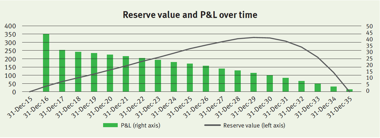
Onwards
The policy will evolve over time as expected, meaning that mortality will be realized as expected and discount rates do not change anymore. The reserve value and P&L over time will evolve as illustrated below.
The profit gradually decreases over time in line with the insurance coverage (i.e. outstanding notional of the mortgage). The relatively high profit in 2016 is (mainly) the result of the realized mortality that was lower than expected (step 2 described above).
As described before, under the full retrospective application, the insurer would be required to go all the way back to the initial recognition to measure the CSM and all consecutive changes. This would require insurers to deep-dive back into their policy administration systems. This has been acknowledged by the IASB by allowing insurers to implement the standards three years after final publication. Insurers will have to undertake a huge amount of operational effort and have already started with their impact analyses. In particular, the risk adjustment seems a challenging topic that requires an understanding of the capital models of the insurer.
Zanders can support in these qualitative analyses and can rely on its past experience with the implementation of Solvency II.


Although the general accounting mechanisms will largely remain unchanged, the long waited reforms of IFRS 9 encompass an array of changes that will influence your hedge accounting process in different ways.
Cross-currency interest rate swaps (CC-IRS), options, FX forwards and commodity trades are just a few examples of financial instruments which will be affected by the upcoming changes. The time value, forward points and cross-currency basis spread will receive different accounting treatment under IFRS 9. Within Zanders, we feel the need to clarify these key changes that deserve as much awareness as possible.
1. Accounting for the forward element in foreign currency forwards
Each FX forward contract possesses a spot and forward element. The forward element represents the interest rate differential between the two currencies. Under IFRS 9 (similar to IAS 39), it is allowed to designate the entire contract or just the spot component as the hedging instrument. When designating the spot component only, the change in fair value of the forward element is recognised in OCI and accumulated in a separate component of equity. Simultaneously, the fair value of the forward points at initial recognition is amortised, most expected linearly, over the life of the hedge.
Again, this accounting treatment is only allowed in case the critical terms are aligned (similar). If at inception the actual value of the forward element exceeds the aligned value, changes in the fair value based on the aligned item will go through OCI. The difference between the fair value of the actual and aligned forward elements is recognized in P&L. In case the value of the aligned forward element exceeds the actual value at inception, changes in fair value are based on the lower of aligned versus actual and go to OCI. The remaining change of actual will be recognized in P&L.
Please refer to the example below:
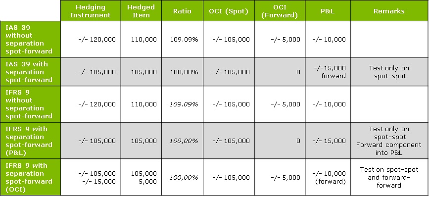
In this example, we consider an entity X which is hedging a future receivable with an FX forward contract.
MtM change of the forward = 105,000 (spot element) + 15,000 (forward element) = 120,000.
MtM change of the hedged item = 105,000 (spot element) + 5,000 (forward element) = 110,000.
We look at alternatives under IAS39 and IFRS9 that show different accounting methods depending on the separation between the spot and forward rates.
Under IAS39 and without a spot/forward separation, the hedging instrument represents the sum of the spot and the forward element (105 000 spot + 15 000 forward= 120 000). The hedged item consisting of 105 000 spot element and 5 000 forward element and the hedge ratio being within the boundaries, the minimum between the hedging instrument and hedged item is listed as OCI, and the difference between the hedging instrument and the hedged item goes to the P&L.
However, with the spot/forward separation under IAS39, the forward component is not included in the hedging relationship and is therefore taken straight to the P&L. Everything that exceeds the movement of the hedged item is considered as an “over hedge” and will be booked in P&L.
Line 3 and 4 under IFRS9 characterise comparable registration practices than under IAS39. The changes come in when we examine line 5, where the forward element of 5 000 can be registered as OCI. In this case, a test on both the spot and the forward element is performed, compared to the previous line where only one test takes place.
2. Rebalancing in a commodity hedge relation
Under influence of changing economic circumstances, it could be necessary to change the hedge ratio, i.e. the ratio between the amount of hedged item and the amount of hedging instruments. Under IAS 39, changes to a hedge ratio require the entity to discontinue hedge accounting and restart with a new hedging relationship that captures the desired changes. The IFRS 9 hedge accounting model allows you to refine your hedge ratio without having to discontinue the hedge relationship. This can be achieved by rebalancing.
Rebalancing is possible if there is a situation where the change in the relationship of the hedging instrument and the hedged item can be compensated by adjusting the hedge ratio. The hedge ratio can be adjusted by increasing or decreasing either the number of designated hedging instruments or hedged items.
When rebalancing a hedging relationship, an entity must update its documentation of the analysis of the sources of hedge ineffectiveness that are expected to affect the hedging relationship during its remaining term.
Please refer to the example below:
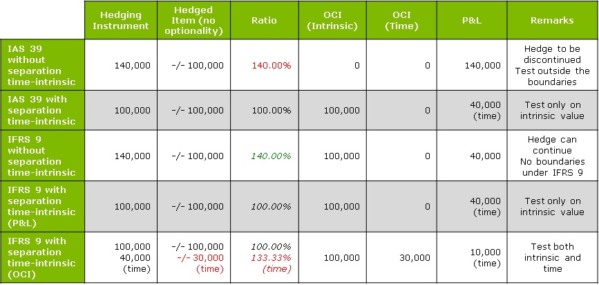
Entity X is hedging a forecast receivable with a FX call.
MtM change of the option = 100,000 (intrinsic value) + 40,000 (time value) = 140,000.
MtM change of the hedged item = 100,000 (intrinsic value) + 30,000 (time value) = 130,000.
In example 3, we consider entity X to be hedging a forecast receivable via an FX call. Note that under IAS39 the hedged item cannot contain an optionality if this optionality is not present in the underlying exposure. Hence, in this example, the hedged item cannot contain any time value. The time value of 30,000 can be used under IFRS9, but only by means of a separate test (see row 5).
In line 1, we can see that without a time-intrinsic separation, the hedge relationship is no longer within the 80-125% boundary; therefore, it needs to be discontinued and the full MtM has to be booked in the P&L. In line 2, there is a time-intrinsic separation, and the 40 000 representing the time value of the option are not included in the hedge relationship, meaning that they go straight to the P&L.
Under IFRS9 with no time-intrinsic separation (line 3), the hedging relationship is accounted for in the usual manner, as the ineffectiveness boundary is not applicable, with 100 000 going representing OCI, and the over hedged 40 000 going to the P&L.
However, the time-intrinsic separation under IFRS9 in line 4 is similar to line 2 under IAS39, in which we choose to immediately remove the time value for the option from the hedging relationship. We therefore have to account for 40 000 of time value in the P&L.
In the last line, we separate between time and intrinsic values, but the time value of the option is aimed to be booked into OCI. In this case, a test on both the intrinsic and the time element is performed. We can therefore comprise 100 000 in the intrinsic OCI, 30 000 in the time OCI, and 10 000 as an over hedge in the P&L.
4. Cross-currency basis spread are considered a cost of hedging
The cross-currency basis spread can be defined as the liquidity premium of one currency over the other. This premium applies to exchanges of currencies in the future, e.g. a hedging instrument like an FX forward contract. If a cross currency interest rate swap is used in combination with a single currency hedged item, for which this spread is not relevant, hedge ineffectiveness could arise.
In order to cope with this mismatch, it has been decided to expand the requirements regarding the costs of hedging. Hedging costs can be seen as cost incurred to protect against unfavourable changes. Similar to the accounting for the forward element of the forward rate, an entity can exclude the cross-currency basis spread and account for it separately when designating a hedging instrument. In case a hypothetical derivative is used, the same principle applies. IFRS 9 states that the hypothetical derivative cannot include features that do not exist in the hedged item. Consequently, cross-currency basis spread cannot be part of the hypothetical derivative in the previously mentioned case. This means that hedge ineffectiveness will exist.
Please refer to the example below:
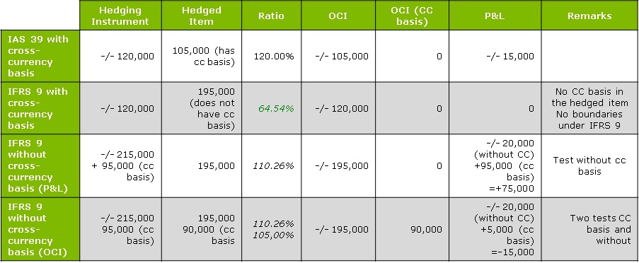
In example 4, we consider an entity X hedging a USD loan with a CCIRS.
MtM change of CCIRS = 215,000 – 95,000 (cross-currency basis) = 120,000.
MtM change hedged = 195,000 – 90,000 (cross-currency basis) = 105,000.
Under IAS39, there is only one way to account for CCIRS. The full amount of 120 000 (including the – 95 000 cross-currency basis) is considered as the hedging instrument, meaning that 105 000 can be listed as OCI and 15 000 of over hedge have to go to the P&L.
Under IFRS9, there is the option to exclude the cross-currency basis and account for it separately.
In line 2, we can see the conditions under IFRS9 when a cross-currency basis is included: the cross-currency basis cannot be comprised in the hedged item, so there is an under hedge of 75 000.
In line 3, we exclude the cross-currency basis from the test for the hedging instrument. By registering the MtM movement of 195 000 as OCI, we then account for the 95 000 of cross-currency basis, as well as -/- 20 000 of over hedge in the P&L. In line 4, the cross-currency basis is included in a separate hedge relationship – we therefore perform an extra test on the cross-currency basis (aligned versus actual values) . From the first test, -/- 195,000 is registered as OCI and -/- 20,000 (“over hedge” part) in P&L; from the cross-currency basis test 90,000 represents OCI and 5,000 has to be included in P&L.

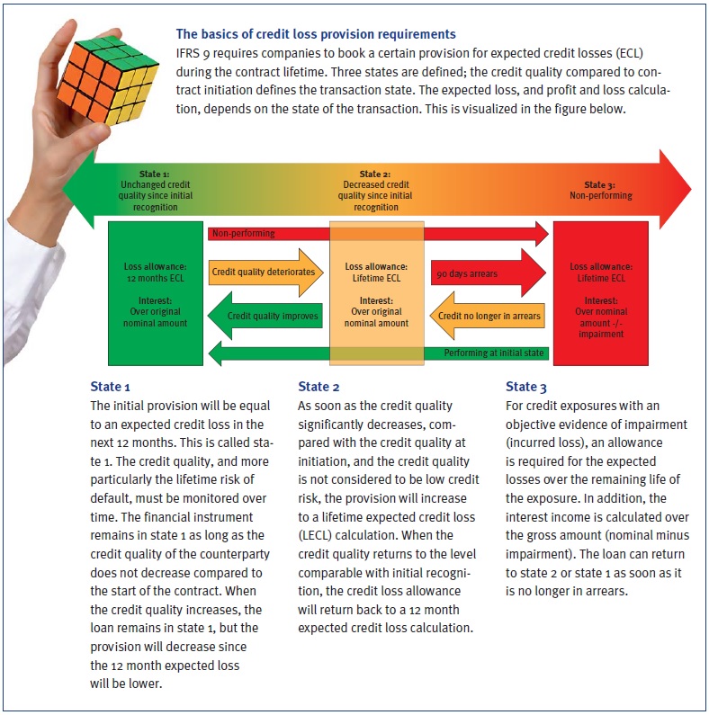
As of January 2018, new accounting rules will come into effect for financial institutions and listed companies with respect to the measurement of impairments. So far, only a few banks act as early adaptors; most choose to be late followers and ‘watch the hare running’. The new rules are principle-based and simple. The design and implementation, however, can be challenging, especially the treatment of forward-looking aspects.
Most banks are struggling to work out how to implement the new impairment rules. Uncertainty over how to deal with current expected credit loss taking into account future macroeconomic scenarios as required by IFRS 9, means credit risk modeling experts, quants and finance experts are in uncharted waters. Different firms have different options on the matter. The primary objective of accounting standards is to provide financial information that stakeholders find useful when making decisions. The new accounting rules regarding provisions will make reserves more timely and sufficient. However, with the new standard, banks are squeezed between P&L volatility, model risk, macroeconomic forecasting and compliance with accounting standards.
Impact
IFRS 9 will, amongst others, rock the balance sheet, affect business models, risk awareness, processes, analytics, data and systems across several dimensions.
We will name a few related to the financials:
- Transition from IAS 39 to IFRS 9 will lead to a change in the level of provision for credit losses. The transition of the current provisions, which are based only on actual losses and incurred but not reported (IBNR) losses, to an expected loss is likely to have significant impact on shareholder equity, net income and capital ratios.
- P&L volatility is expected to increase after transition, since deterioration in credit quality or changes in expected credit loss will have a direct impact on P&L. The P&L volatility will, however, significantly differ per type of credit portfolio, also depending on counterparty ratings and remaining maturity. Portfolios with loans rated below investment grade will move faster from ‘state 1’ to ‘state 2’ (see box), since a move within investment grade ratings is not seen as a credit quality deterioration. Portfolios with long maturities will face large P&L volatility when moving from state 1 to state 2.
- Capital levels and deal pricing will be affected by the expected provisions.
Total P&L over time will not change, since the expected credit loss provision is booked against the actual credit losses during lifetime. If there is no actual credit loss, all provisions will fall free as profit towards maturity.
Forward-looking
IFRS 9 requires financial institutions to adjust the current backward-looking incurred loss based credit provision into a forward-looking expected credit loss. This sounds logical for an accounting provision and it assumes that existing relevant models within risk management may be applied. However, there are some difficulties to overcome.
Incorporating forward-looking information means moving away from the through-the-cycle approach towards an estimation of the ‘business cycle’ of potential credit losses. A forward-looking expected credit loss calculation should be based on an accurate estimation of current and future probability of default (PD), exposure at default (EAD), loss given default (LGD), and discount factors. Discount factors according to IFRS 9 are based on the effective interest rate; this subject will not be further addressed here. The EAD can mainly be derived from current exposure, contractual cash flows and an estimate of unscheduled repayments and an expectation of the use of undrawn credit limits. Both unscheduled repayments and undrawn amounts are known to be business cycle dependent. Forecasting these items can be derived from historical observations.

Of course, the best calibration is on defaulted data since we determine exposure at default. If insufficient data is available, cycle dependent unscheduled repayments and drawing of credit limits can be derived from the entire credit portfolio, preferably corrected with some expert judgement to reflect the situation at default.
Banks have internal rating models in place to assign a PD to a counterparty and for trenching the portfolio in different levels with a specific PD. From a capital point of view, these ratings are mostly calibrated to a through-the-cycle level of observed defaults. Now using all the bank’s forward-looking information may improve estimates if business cycle(s) can be identified, potential scenarios of the development of the cycle in the future can be forecasted, including how the cycle affects a bank’s PD term structure. This would be a macroeconomic and econometric heaven if there were sufficient data available to derive accurate and statistically significant models. Otherwise, banks need to rely more on expert judgement and external macroeconomic reports.
Next to the PD term structures, LGD term structures are required to calculate a life time expected loss. Deriving an accurate LGD term structure from realized defaults requires a large default database. Deriving a business-cycle dependent LGD term structure requires an even bigger database of accurately and timely documented losses. The level of business cycle dependency of LGD significantly differs per type of counterparty, industry, and collateral. Subordination is not much cycle dependent, while loans covered with collateral, such as mortgage loans, may result in large movements in LGDs over time. Hence, this requires different LGD term structures for different LGD types and levels.
Economic scenarios
Incorporating forward-looking information means modeling business cycle dependency in your PD and LGD. For significant drivers, future scenarios are required to calculate expected credit loss. At most banks, these forward-looking scenarios are commonly the domain of economic research departments. Macroeconomic forecasting concentrates mainly on country-specific variables. Growth of domestic product, unemployment rates, inflation indices and interest rates are typical projected variables.
Usually, only large international banks with an economic research department are able to project consistent economic outlooks and scenarios. Next to macro scenarios, industry specific forecasts are important. Industry risk models enable a bank to make forecasts for a certain industry segment, e.g. chemicals, automotive or oil & gas. Industry models are often based on variables such as market conditions, barriers to entry and default data. At some banks, industries are analyzed and scored by economic researchers. At others, usually smaller banks, industries are ranked by sector business specialists.
Industry scorings often form input for rating models and are important factors for portfolio management purposes. Therefore, caution is required in correlation between drivers of ratings and drivers of the PD term structure.
Credit portfolios
For homogenous retail exposures, forward-looking elements can be considered on a portfolio level by modeling the dependencies of PD and LGD percentages for realized defaults and losses; in essence this is a bottom-up approach. For mortgage portfolios, cycle dependency relates, for example, to unemployment and house price indices, among other factors. However, statistically significant parameters and models for default relations are difficult to obtain since there is a common time gap in observing and administrating both defaults and business cycle.
Model significance can be improved by adding additional variables with increasing risk of overfitting. Even if there is statistical proof for macroeconomic dependencies in PD and LGD rates, it is advised to be cautious, since it also requires designing credible macroeconomic scenarios. As business cycles are difficult to predict, this could lead to extra P&L volatility and an increase in the complexity and ‘explainability’ of figures. Therefore, regular back-testing and continuous monitoring are important for an accurate and robust provision mechanism, especially in the first years after the model is introduced.
For non-retail exposures, country and industry risk are, if embedded in the credit rating models, already part of the annual individual credit review and rating assignment processes. In the monthly financial reporting, additional country and industry risk factors can be taken into account on a portfolio basis, making provisions more forward looking; in essence a top-down approach. If necessary, risk management can make adjustments on an individual basis for wholesale counterparties, and facilities. A forward-looking overlay should improve the accuracy of provisions and a timely and adequate recognition of credit risk, instead of “too little, too late” as under the existing rules.
Governance
Because of the forward-looking character of IFRS 9, and the increasing role of risk models, a transparent and robust governance framework will become more important. Coordination and communication are required across risk, finance, business units, audit and IT.
Risk management typically delivers the expected credit loss parameters and calculations to finance on a monthly basis. Proposals for retail and nonretail adjustments briefly described above, must be discussed and agreed upon, after which the final proposal is submitted to the approval authority.
The governance framework should be documented and reviewed on an annual basis, and highlight key functions, stakeholders, definitions, data management, model (re)development, model implementation, portfolio monitoring and validation. In addition, all parties involved should speak the same credit risk language, have access to detailed data underlying the calculation of the provision and a good under- standing of the model and implications of decisions and parametrization. Only then can the finance department obtain an accurate understanding of the level and change of the provision and clearly inform the board and other stakeholders.
Zanders recommends preparing early for IFRS 9 and having a deep and thorough understanding of the impact, as well as the robust tooling and processes in place. Don’t just wait and ‘watch the hare running’, but start early, and at least run a shadow period during daylight to allow sufficient time.
Hassle-free CECL and IFRS9 compliance? Try our new Condor ECL tool!


