Criminals never stand still, and neither should the models designed to catch them. Across the financial sector, institutions have invested heavily in advanced Financial Crime Prevention (FCP) models to detect fraud and money laundering. Yet the environment these models operate in is evolving faster than ever. As new technologies emerge and criminal behaviors adapt, yesterday’s patterns no longer predict tomorrow’s risks. 

Take cryptocurrencies: once niche, now mainstream. Their rise has transformed what “normal” transactions look like, blurring the line between legitimate activity and illicit movement. This shift underscores a growing challenge for banks—model drift. Without continuous monitoring and recalibration, even the most sophisticated FCP models can lose accuracy and allow financial crime to slip through the cracks. 

Model Drift, Data Drift, Concept Drift – What Are They? 

Model drift is defined as the degradation of the model’s performance over time. This can be due to many factors, such as sampling bias, but also due to data drift or concept drift. Data drift and concept drift are related and occur often at the same time, but tackle a different underlying issue.  

Data drift occurs when the distribution of data underlying your model changes. Take for example, bank A which acquires bank B. Such a takeover might change the underlying customer base significantly. Assuming that bank B has a higher risk appetite, these clients likely require different monitoring from the original customer base, e.g. by changing thresholds or developing new rules. 

Concept drift on the other hand means that a relationship that a model presupposes deteriorates or does not exist anymore. This can have large effects on the quality of model predictions. For example, criminals continuously develop new money laundering tactics to avoid being detected by ever-improving transaction monitoring models without impacting overall transaction distributions. This way the model still detects the outdated method the criminals used to apply but not the new methods. As a result, the model decreases in effectiveness. 

As mentioned above, data drift and concept drift often occur together. An example of these two concepts coming together is for the aforementioned cryptocurrencies. The distribution of cryptocurrencies have shifted significantly with more and larger transactions indicating data drift. In addition cryptocurrencies have gained a lot of popularity amongst criminals for developing new money-laundering schemes indicating concept drift. 

How To Monitor Model Drift 

Both concept and data drift can occur after the go-live of the model. It is crucial to have proper monitoring in place to timely be alerted. Generally, model monitoring frameworks include periodic review of a models’ effectiveness. Creating awareness for data drift and concept drift during this periodic review can create an alertness if the model performance or underlying distribution significantly shifts. Besides the regular assessment cycle, some monitoring thresholds can be upheld: 

• Data drift: measure the underlying distribution of risk drivers at model initiation. Significant distortions in this initial distribution should be bound to some pre-defined limit. Once these thresholds are breached, a review can be initiated to assess its contribution in erroneous predictions. An example of a metric that could be used for this purpose is the Population Stability Index (PSI), which measures the difference between the distributions of two different population samples. 

• Concept drift: measure the predictive power of the individual risk drivers against the dependent variable. If there seems to be significant deterioration of the explanatory power, a review of the model design can be initiated. For example by using SHAP-values, the individual contribution of a risk driver towards the general risk classification can be utilized. If these SHAP-values provide a decrease in explanatory power since model initiation, this can indicate concept drift. 

Prevent Drift From Derailing Your Models 

Besides a solid model monitoring framework and regular periodic reviews of the model, model drift should also be considered during model development. During model (re)development, the following points should be considered to counteract model drift: 

• Measure the sensitivity of the model against small changes in averages of your input. Assessment of the impact of changes in individual risk drivers can give insight into over-reliance towards specific characteristics that are prone to change.  

• Sensitivity can also be measured towards the change in distribution, such as flattening or skewing the distribution.  

• Assess the change to your model when risk drivers are removed. Here, again, the impact should be manageable.  

• Investigate the stability of your risk drivers over time.  

• Perform a qualitative analysis on the robustness of risk drivers. 

These steps give a solid base to include mitigants for data drift and concept drift into your model development cycle. 

This article is part of a larger series highlighting crucial topics for the future of financial crime prevention. See an overview of the whole series here. 

Creating a solid model development framework that includes model and data drift can be a challenge and requires deep domain experience and experience. If you need guidance in making your models future-proof, Zanders can help.  

Want to know how Zanders can support you in this transition? Feel free to reach out through our contact page to get in touch with an expert.  

AI is everywhere – but many treasurers still struggle to move beyond the hype and identify real, value-adding applications. That’s why in this blog series, we’ll explore four practical use cases in depth, each resulting in a concrete, actionable application you could begin implementing tomorrow. 

In this blog, we focus on one of the most time-consuming challenges in any treasury transformation: system testing. Testing remains highly manual, repetitive, and resource-intensive. But the rise of AI agents is changing the game, offering a way to make testing faster, more intuitive, and highly repeatable. 

The Challenge 

Testing is at the heart of every treasury transformation. It’s a meticulous, iterative process: before you even begin, you need a robust set of test cases that reflects your specific workflow to ensure every critical scenario is covered, without drowning in an endless list. Then comes the manual execution, documentation, and feedback cycles, repeated again and again until every issue is resolved. 

Even after go-live, the work isn’t over. Regular system updates and configuration changes mean more rounds of regression testing to catch any unexpected side effects. It’s essential work, but it can be a real drain on time and resources. 

Now, thanks to AI, there’s a smarter way. 

The Solution 

You are currently viewing a placeholder content from YouTube. To access the actual content, click the button below. Please note that doing so will share data with third-party providers.

More Information

Unblock content Accept required service and unblock content

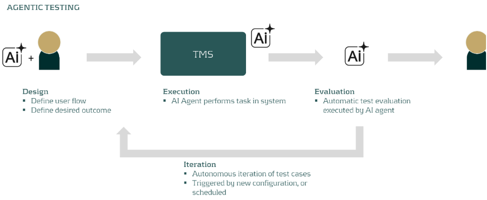
AI agents are autonomous actors that can interact directly with your web browser and through that with your Treasury Management System (TMS) to complete tasks and resolve issues. Imagine instructing an AI agent in plain language, and watching it execute complex test cases right in the user interface. The agent is able to navigate to the right page, fill in information in the forms, the buttons, and record output. The flexibility of these agents even allow them to identify error messages and validate the result of a set of actions.  

Armed with vendor documentation, solution designs, and implementation blueprints, the AI agent proposes a comprehensive set of test cases and relates those to actions in your system of choice. Users can easily add their own scenarios by simply describing the workflow. The agent then navigates the system, executes the tests, and records the results, all autonomously. 

Worried about safety? Don’t be. Today’s test automation tools come with robust guardrails: 

• Test environments only: No risk to production. 

• Controlled user rights: The agent gets only the permissions it needs. 

• Plan mode: The agent presents its action plan for human approval before anything runs. 

With these safeguards, the risk of unintended actions is virtually eliminated—while the efficiency gains are game-changing. 

You can build AI agents in-house, but many organizations will benefit even more from cloud-based platforms. These solutions: 

• Lower deployment costs and speed up implementation 

• Offer ready-made integrations 

• Enable users to share successful test scenarios 

At Zanders, we’ve developed an AI-powered test suite that plugs directly into leading cloud TMS platforms—empowering treasurers to accelerate testing without sacrificing control. 

A Real-World Example 

Let’s make this tangible. Suppose you want to test a workflow for adjusting FX exposure and generating a report. The AI agent, using system documentation and blueprints, proposes relevant user flows. One test case might be: 
“Change the EUR/USD exchange rate to 1.12, create a new EUR/USD FX Forward with a six-month maturity, and run the FX Exposure report.” 

The agent executes these steps, records the results, and once the optimal route is captured, can repeat the test autonomously and even evaluate the outputs itself. Over time, you build a powerful, reusable suite of automated test scenarios for both transformation projects and ongoing regression testing. 

Conclusion 

AI in treasury is no longer a futuristic possibility, it’s a practical, high-impact technology that treasury teams can start leveraging today. Do you want to explore automated testing? Contact us! Are you interested in other concrete use cases, learn more about transforming your treasury operations for the digital age. 

In the pursuit of climate-aligned finance, financial institutions face a critical challenge: incomplete emissions data. While disclosure frameworks such as the EBA’s Pillar 3 ESG requirements, the ECB’s climate risk guidance, and the EU Corporate Sustainability Reporting Directive (CSRD) continue to expand, their scope remains fragmented. Therefore, financial institutions must often assess climate-related financial risks and align portfolios without full visibility into counterparties’ environmental footprints.  

In collaboration with a leading international bank, Zanders explored how machine learning can support more accurate, scalable, and decision-useful estimates of greenhouse gas (GHG) emissions intensity when disclosures fall short. 

The Challenge: Incomplete GHG Emissions Disclosure 

Current climate risk assessments rely heavily on firm-disclosed emissions. Yet, many companies, particularly small, private, or non-European, still do not report their GHG emissions. This inconsistency not only limits the accuracy of portfolio-level financed emissions metrics, but also hinders accurate net-zero alignment tracking and regulatory reporting. 

To fill this gap, many financial institutions resort to sector-average proxies, such as those recommended by the Partnership for Carbon Accounting Financials (PCAF). These proxies assign emissions to non-reporting firms based on average industry and regional emission intensities. While widely adopted, this approach introduces substantial bias, as it overlooks firm-specific drivers such as energy use, capital intensity, or geographic differences. The result is a blind spot: portfolio assessment loses the very granularity needed to distinguish leaders from laggards in the low-carbon transition. 

Predicting Emissions Intensity with Machine Learning 

The main objective of the study focused on testing various supervised ML models to estimate Scope 1 and 2 GHG emissions intensity based on a variety of financial firm-level characteristics. Leveraging an unbalanced panel dataset covering worldwide public and private companies from 2021 to 2025, models were trained to learn from disclosed emissions and predict missing values with greater granularity. The dataset was split into approximately 80 % training and 20 % testing subsets, ensuring that observations from the same company (across different years) did not appear in both sets to prevent information leakage. 

Two models were introduced: 

• Model 1, a baseline that includes financial and sectoral indicators widely available for banks, such as assets turnover; property, plant and equipment (PPE); earnings before interest and taxes (EBIT); and industry classification.  

• Model 2, an extended model that incorporates more advanced and less common variables such as Refinitiv ESG score; energy consumption; and earnings quality rankings. 

These predictors were selected based on both academic relevance and practical availability in financial databases such as LSEG Workspace (previous Refinitiv Eikon) and S&P.  

In both Model 1 and Model 2 settings, three algorithms were compared: k-Nearest Neighbours (k-NN), Decision Trees, and Random Forests, chosen for their interpretability and practicality in low-data environments. To assess whether machine learning provides a meaningful improvement over traditional sector-average proxies, both the ML models and PCAF sector-average proxy estimates were examined on a common test set. Unification of this comparison allowed for quantifying the overall predictive gains and evaluating the implications for climate-aligned decision-making in finance. 

Models performance was evaluated using standard regression metrics including Root Mean Squared Error (RMSE), and Mean Absolute Error (MAE), ensuring consistency across models and comparison with the baseline. Beyond standard error metrics, performance was also assessed through variance recovery (reported further as Median Variance Relative Gain). This measure captures how effectively each model restores firm-level differentiation in GHG emissions intensity lost under sector-average proxies.  

The entire framework was designed to balance predictive accuracy with implementation realism, aiming to improve GHG coverage for financial institutions without relying on black-box techniques or data-heavy infrastructure. 

What the Models Revealed 

Under each model and method, machine learning substantially outperformed the traditional PCAF proxy approach: 

The Random Forest version of Model 2 emerged as the strongest performer, reducing RMSE by roughly one-third, MAE by more than a half and recovering nearly 65% of the intra-sectoral variance lost under sector-average proxies. Model 1, created for banking sector usage, scored a second place under the same Random Forest algorithm, reducing RMSE by 21% and MAE by 41%. This means that the algorithm can effectively differentiate firms within the same industry, being a critical step for a realistic transition-risk modeling or portfolio creation. 

Feature importance analysis showed that Energy Use Total, PPE / Total Assets, Asset Turnover and Sector were consistently dominant predictors, confirming that emissions intensity depends jointly on operational efficiency and capital structure. However, the study also tested a transfer learning approach, where models trained only on high-disclosure sectors with sufficient reporting coverage were applied to low-disclosure sectors, unseen during training. The results showed a substantial decline in accuracy, suggesting that emission patterns are highly sector specific. In practice, this means that for ML models to exceed sector-average proxies in the GHG emission estimation context, models should be trained on datasets that include all sectors, rather than relying on samples limited to a few well-disclosing industries. 

Why This Matters 

More accurate emissions estimation directly supports key pillars of sustainable finance. It enhances portfolio alignment assessments, scenario analysis, and climate risk disclosure under frameworks such as Task Force on Climate-related Financial Disclosures (TCFD) and the EU Corporate Sustainability Reporting Directive (CSRD). Moreover, improved firm-level granularity enables financial institutions to better understand which clients are leading or lagging in the transition to a low-carbon economy. 

By replacing rigid proxies with data-driven predictions, financial institutions can move one step closer to climate data maturity, where decisions are no longer held back by disclosure gaps but empowered by intelligent estimation. 

What Zanders Can Do 

As regulatory expectations tighten and data coverage remains incomplete, financial institutions need solutions that are both technically rigorous and operationally feasible. Whether addressing climate-related credit exposures, integrating ESG into portfolio construction, or navigating disclosure obligations, institutions must adopt frameworks that are adaptive, data-driven, and aligned with supervisory standards. 

By combining quantitative modeling expertise, climate risk analytics, and regulatory knowledge, Zanders helps institutions move beyond generic estimates and static proxies. 

Want to find out more about how we can support you in building practical ESG risk management solutions? Our ESG experts will be happy to assist you. Visit the Zanders ESG page to know more. 

For many companies, especially in regulated industries like finance, the fear of AI is not just philosophical; it’s a practical challenge. It stems from a perceived loss of control, a lack of transparency, and the worry that decisions made by complex models might be difficult to justify to regulators, auditors, or the public. 

This fear is understandable. When machine learning models autonomously flag transactions, deny loans, or possibly even escalate alerts to authorities, the stakes are high. The consequences affect not just business outcomes, but reputations, regulatory standing, and real people’s lives. In Financial Crime Prevention (FCP), where analysts must decide whether to file a Suspicious Activity Report (SAR), the need for clarity is of great importance. 

This fear doesn’t have to mean that these models have no place in these departments. Rather, it can guide us to the correct place. The focus should shift from: "how the model works" to: "how the model helps."  

Empowering Analysts

In AI deployments, explainability is treated as a technical afterthought, a set of metrics or plots that satisfy internal documentation or regulatory checklists. But in FCP, the true end-user of an AI system is the analyst. They are the ones who must interpret alerts, justify decisions, and ensure compliance. Their job is not to understand gradient boosting or SHAP values, analysts should have a focus  to make the results defensible and take informed decisions under pressure. 

Human-centered explainability means designing explanations that support this task. It’s not about simplifying for the sake of clarity, it’s about making the explanation meaningful and relevant to the task at hand. This approach should turn the model from a black box into a collaborative partner. 

Instead of presenting abstract SHAP plots, one could consider: 

• Top contributing risk factors for each alert, along with an explanation of what each factor represents. While most models already use feature importance to describe their behavior, analysts tend to interpret these factors from a risk perspective. A simple way would be providing a mapping between model features and risk indicators which could help analysts better understand what drives an alert and why it matters. 

• Narrative summaries that explain why a transaction deviates from expected behavior. One could for instance leverage the power of LLM’s for transforming data into plain-language interpretations.  

• Consistency checks that show how similar cases were treated, building trust in the system’s fairness. 

Too often, explainability efforts focus on stakeholders around the model; data scientists, compliance officers, or regulators. But the real test of explainability lies with the analyst who must act on the model’s output. By centering design on their needs, we shift the conversation from how the model works to how the model helps. 

This shift doesn’t just improve usability; it builds trust. And in a domain like FCP, trust is everything. 

Explainability as a Bridge, not a Barrier 

AI continues to be a sensitive topic in the risk-conscious world of Financial Crime Prevention, largely because its explainability focuses heavily on technical model details. But the real value of AI lies in how it supports analysts, helping them interpret alerts, make informed decisions, and justify their actions with confidence. That’s why explainability should be designed with the analyst in mind. By doing this, AI becomes not only more transparent, but also more useful, more responsible, and more trusted. 

Understanding and applying explainability metrics in Financial Crime Prevention (FCP) is no longer just a technical exercise, but a human-centered challenge.  

As highlighted in our blog series on the future of FCP, explainability is just one of the critical pillars shaping responsible AI adoption in this domain. If you're navigating the complexities of explainability and wanting to ensure your AI systems are not only compliant but also trusted and usable by those on the front lines, Zanders can help. 

In recent years, bias¹ and fairness in AI models have become critical topics of discussion, especially as algorithmic decision-making has led to unintended and sometimes harmful consequences for specific groups. Notable examples include the “Toeslagenaffaire “ in The Netherlands (Toeslagenaffaire) and the COMPAS case in the United States (COMPAS case). Both of these examples highlight how models that include algorithmic decision making can display unwanted bias without proper governance.  

In the Financial Crime Prevention (FCP) domain, AI models are often used to detect criminal behaviour such as fraudulent transactions, money laundering, and tax evasion. These models are not just operational tools – they are subject to regulation. For instance, National Central Banks may mandate that banks demonstrate sufficient effort in identifying financial crime (The DNB on Money Laundering and combating criminal money), with penalties for underperformance. Performance is typically measured using (a derivative of) recall², which measures the model’s ability to identify as many true cases of criminal behaviour as possible. 

Recently, several Dutch banks faced fines from regulators for failing to meet these requirements, underscoring the pressure to maximize recall.  

However, this focus on maximizing recall must be balanced with fairness. Regulators also require banks to detect and mitigate unwanted bias in their models (EBA report, AI Act), which relates to the metric precision² – the proportion of flagged cases that are actually criminal. A low precision rate can result in clients being wrongly flagged, which raises ethical and legal concerns. 

The Pitfalls of Conventional Bias Fixes 

Assessing the fairness of a model typically includes comparing precision-like metrics across different groups with similar sensitive information (e.g., groups based on gender or ethnicity). If significant disparities are observed between groups, steps are typically taken to align the precision values more closely. While this approach is popular and intuitive, it comes with several challenges: 

1. Conflicting objectives: Precision and recall are inherently at odds. Optimizing for one generally compromises the other. Banks must navigate regulatory demands for high recall while also ensuring fair treatment across groups, with no established best practices to guide these trade-offs. 
2. Levelling down: Achieving equal precision across groups can involve either improving the disadvantaged group's performance or reducing the advantaged group's performance. In practice, improving precision for disadvantaged groups is often infeasible due to limited data or inconsistent behavioural patterns. This leads to "levelling down" – artificially lowering the precision of the advantaged group to achieve parity (The Unfairness of Fair Machine Learning: Levelling down and strict egalitarianism by default). While this may equalize precision metrics, it does not improve outcomes for the disadvantaged group and often degrades overall model performance. Therefore, whether this approach is truly fair remains a subject of debate.  
   
   In the context of FCP, one could challenge the assumption that the goal should be to achieve strict statistical parity between groups at the cost of lower recall. For a model that e.g. detects fraudulent transactions, achieving strict parity by decreasing the recall for advantaged groups could be considered inappropriate, with potentially harmful societal consequences. Levelling down is a classic example of Goodhart’s Law that “when a measure becomes a target, it ceases to be a good measure”.  
   
   
3. Use of sensitive information: Testing for unwanted model bias usually involves customer segmentation based on sensitive attributes. However, this process can lead to the sensitive data being used in the model development process, either directly (e.g., as input features) or indirectly (e.g., through group-specific decision rules or parameters). Under the General Data Protection Regulation (GDPR), this is generally prohibited.  

Potential Next Steps 

Bias and fairness considerations, especially within Financial Crime Prevention, require moving beyond the simple pursuit of strict statistical parity. In addition to established practices, more nuanced and responsible approaches should be considered:   

• Establish a bank-wide “bias and fairness” committee: Create a bank-wide diverse committee consisting of experts across different departments such as modeling & data, compliance, and risk. This committee should define unified fairness principles, oversee their consistent application across departments, and act as a governance hub for addressing emerging fairness concerns in AI-driven decision-making. 

• Develop an impact-based fairness framework: Move beyond solely equalizing metrics by building a framework that measures the tangible impact of bias on different customer groups. This enables institutions to focus resources where potential harm is greatest, ensuring fairness interventions deliver meaningful outcomes. 

• Leverage explainability tools to detect hidden biases: Tools like SHapley Additive exPlanations (SHAP) are commonly used to meet regulatory requirements regarding explainability. Beyond compliance, SHAP can also help uncover which (combinations of) features act as proxies for sensitive attributes like gender or ethnicity. This could help to proactively detect hidden biases and strengthen fairness in FCP models. 

This article is part of a larger series highlighting crucial topics for the future of financial crime prevention. See an overview of the whole series here. 

Navigating the complex ecosystem of bias and fairness metrics in the context of FCP demands deep domain expertise and a clear understanding of the regulatory and ethical landscape. If you need guidance in translating complex fairness metrics into actionable, compliant, and effective practices, Zanders can help.

The interest in AI has been increasing at record pace, with new technology releases every month and an impressive number of new use cases for chatbots or agents. However, many treasurers still struggle to translate this hype into value-added implementations for their business. These upcoming blog series explore practical use cases for AI that delivers concrete value to treasurers. This article specifically shares an implementation of AI agents to automate the pricing, review and documentation of intercompany loans.

The challenge

One of the core functions for many treasury departments is the distribution of cash in their group. Intra-group loans are one of the tools used by treasurers to distribute cash, but their use comes with challenges. The interest rate on intercompany loans has a significant impact on the tax expense incurred by the subsidiary and taxable income received by the head-office and therefore should be based on an arm's length approach.

Arm’s length pricing of intercompany loans requires a detailed analysis of the credit standing of the borrower, the influence of the group on the borrower’s credit risk, and a review of the debt market to determine a price. Due to the tax implications, this process should be documented in detail including sources and models. Regulations surrounding transfer pricing of financial transactions have been expanding in many countries in the past years, posing greater challenges for treasury teams to perform a complex process with high compliance requirements. As a result, many have resorted to advisors or build complex Excel models to perform the recurring pricing analyses.

The solution

The main challenge when automating the pricing of intercompany loans is the access to data and models. A compliant process relies on the periodic retrieval of benchmark transactions to set an interest rate – for example with bonds, loans, or a Credit Default Swap (CDS). On the other hand, an objective calculation of the credit risk requires a model that is explainable and is filled with company data.

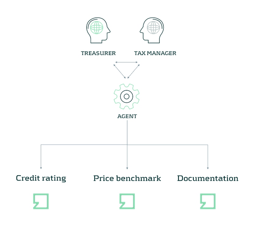
AI Agents are a powerful tool that can be used to automate the retrieval of data and execution of tools in a complex process with changing inputs. In the diagram below, an AI Agent is coupled with a credit rating model, a tool to gather benchmarking data, and a documentation method. In our implementation, we have used the modules in the Zanders Transfer Pricing Solution to provide this functionality to the agent. Next to the tools, it is important to provide the Agent with sufficient context on what role it should play and how it should execute a pricing analysis. The agent should understand the compliance requirements and the tools before it can reliably run the process. For this use case, this is done through context engineering by providing example cases, differences in methods, and checks that the agent should perform.

In the resulting setup, the Agent can automate the full pricing step: identifying entities, calculating a credit rating, and running a pricing benchmark. As a result, the Agent provides a report that is generated according to our template.

With the same tools, we can extend the system even further, by reviewing past calculations versus policies and tax regulations to spot high risk cases or evaluating the credit position of entities to set borrowing limits or update credit ratings. By automating these processes, treasurers can move away from the operational hassle of pricing intercompany loans and instead focus on managing the funding mix of their group. Agents take care of automatic handling of loans and the importing or exporting of data, where treasurers set the objectives of the pricing approach and funding.

AI in Treasury is no longer a futuristic possibility - it's a practical, high-impact technology that Treasury teams can start leveraging today. Do you want to explore intercompany pricing? Let us know in this contact form below.

If you are interested in more use cases, read more here.

As part of the consultation process, open until 29 October 2025, the credit risk specialists at Zanders share our perspective on the proposed guidelines levering on our extensive expertise in credit risk modeling.

Building on existing EBA guidelines on PD and LGD estimation, the new CCF guideline aims to strengthen consistency across all IRB risk parameters. The proposed guideline provides clearer direction and changes on topics such as:

• Level of modeling: facility-level realized CCFs are required, where aggregation possibilities are limited, and fully drawn facilities are explicitly included in scope.
• Realized CCF: a methodology is provided to determine the CCF based on the level of utilisation.

In addition, the guidelines simplify regulatory expectations compared to the Guidelines on PD and LGD estimation such as:

• Representativeness: model performance outweighs representativeness constraints.
• Risk quantification: the long-run average should be the facility-weighted average of realized CCFs.
• Downturn adjustments: only the extrapolation approach is permitted.
• In-default CCF estimation: the methodology for non-defaulted exposures also applies to defaulted exposures.
• Non-retail exposures: under certain conditions a simplified approach allows using the same CCFs for non-defaulted and defaulted exposures, where estimated drawings for unresolved defaults are omitted.

Recognizing the smaller scope of CCF and data availability compared to PD and LGD, the proposed guidelines introduce a more proportionate and pragmatic approach for CCF estimation.

This article highlights these developments, focusing on the level of modeling, the determination of realized CCF, and the simplified approaches to representativeness, risk quantification, and downturn estimation.

Level of Modeling and Application

Under Article 4(1)(56) of the CRR3, institutions are required to calculate the realized CCF at the level of each individual facility for every default. The EBA’s proposed guidelines enforce this requirement by mandating a separate realized CCF for each facility, allowing exceptions only when several revolving limits stem from related contracts linked through an overarching agreement (i.e. umbrella facility with a shared debt ceiling) and have comparable characteristics.

This represents a clear difference from the flexibility allowed under ECB’s Guide to Internal Models (EGIM) paragraphs 259 and 316, which do not require comparability of characteristics. Under EGIM it is allowed to aggregate at a higher level than the individual facility irrespective of product characteristics, such as aggregation when LGD is estimated at a higher level. The proposed EBA guidelines therefore tightens the existing framework by explicitly prohibiting the aggregation of contracts with very different characteristics.

For institutions, this means developing a deeper understanding of the customer’s product structure and closely monitoring changes in the product mix during the twelve months leading up to a default. A facility is in scope of the CCF model if it contains a revolving contract at the reference date. Contracts that become revolving or non-revolving after a restructuring within the same facility are therefore also included. However, repayments on term loans should not impact the CCF, meaning term loans at the reference date should effectively be excluded. Therefore, institutions must continue to track the exposure as part of the original commitment. This can lead to complex situations, as illustrated below. The brown-highlighted contracts (originating from term loans) are out of scope, while the green-highlighted contracts are in scope. The new contract III is considered in scope because it can be interpreted as an increase in the facility limit.

The realized CCF for this facility is calculated as the difference between the drawn amount at the default date (100 + 50) and the drawn amount at the reference date (50) divided by the undrawn amount at the reference date (50) of the contracts in scope. As a result, the realized CCF is ( (100+50)-50) / (100 – 50) = 200%.

Example:

Moreover, when several facilities are backed by the same collateral, they are often combined into a single recovery account during the recovery process (see example below). In such cases, these facilities can be grouped for LGD. Under the EGIM framework, there was flexibility to also aggregate them for CCF modeling. However, the new guidelines require institutions to precisely allocate outstanding amounts to each specific revolving facility that existed at the reference date. This can create inconsistencies between LGD and CCF modeling and adds complexity to the modeling process. As a result, institutions will need to improve their systems to consistently identify, link, allocate, and manage facilities across their portfolios.

Example:

An obligor has an overarching collateral securing two different facilities I and II. Both facilities consist of revolving off-balance sheet exposures, but have different characteristics. During the recovery process, they are combined into a single recovery account. Therefore, all these facilities are grouped for LGD.

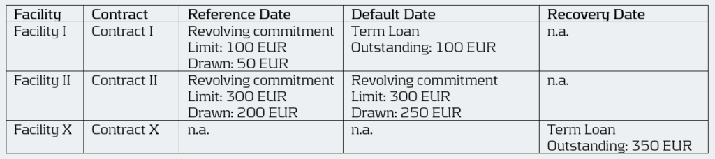
Under EGIM it was permitted to calculate the CCF at the LGD aggregation level, resulting in a realized CCF of ((100 + 250) – (50 + 200)) / ((100+300) – (50+200)) = 66.7%. Under the proposed guidelines, however, the realized CCF must be calculated separately for each facility, giving a CCF of 100% for Facility I (i.e. (100 – 50) / (100 – 50)) and 50% for Facility II (i.e. (250 – 200) / (300 – 200)).

Calculation of Realized CCF

The proposed EBA guidelines introduce two key changes in how institutions determine the realized CCF.

While EGIM paragraph 317 could be interpreted as fully drawn facilities are out of scope, the first change explicitly brings fully drawn revolving commitments into the scope of IRB-CCF modeling, marking another key difference between the two frameworks. EBA’s proposed guidelines now distinguishes between three levels of facility utilization for CCF estimation:

1. Fully drawn facilities.
2. Near-fully drawn facilities, which fall within the so-called Region of Instability (RoI). For example, a facility with a EUR 1000 limit and EUR 995 drawn at the reference date. If an additional EUR 30 is drawn between the reference date and default, the CCF would be: (1020-995)/(1000-995) = 500%.
3. Partially drawn facilities.

The realized CCF is in general determined by the difference in drawn amount at default and the reference date as a percentage of the undrawn amount at the reference date. Since fully drawn facilities have no undrawn part at the reference date, institutions must use an alternative calculation method that expresses the drawn amount at default as a percentage of the committed limit at the reference date. Facilities that are in the RoI, have a very small undrawn amount, which can result in unstable and unreliable realized CCF estimates. Although Basel III describes three possible methods to handle such cases, the guidelines recommend applying the same approach used for fully drawn facilities when predictive accuracy or discriminatory power is limited. They highlight that consistency in applying the chosen approach is essential. Moreover, institutions are expected to define clear thresholds that identify these cases, where it is essential to balance the need to capture outliers without including an excessive number of cases.

The second change concerns the treatment of additional drawings. For retail exposures, institutions retain the flexibility to include additional drawings either in the LGD or in the CCF estimation. For non-retail exposures, additional drawings must still be incorporated into the CCF estimates. In situations where the additional drawings are considered in the CCF all observed drawings should be considered. However, if there are many drawings and repayments, realized CCFs can in practice be very high and LGDs very low (see example below).

Example

The facility has a drawn amount of EUR 100 and a limit of EUR 120, meaning there is an undrawn amount of EUR 20. If the additional drawings would simply be summed, this would lead to a total drawn amount of EUR 60 and a total recovery amount of EUR 160.  As a result, ignoring discounting, this would mean the CCF is EUR 60 / EUR 20 = 300% and the LGD would be ((EUR 100 + EUR 60) – EUR 160) / (EUR 100 + EUR 60) = 0%.

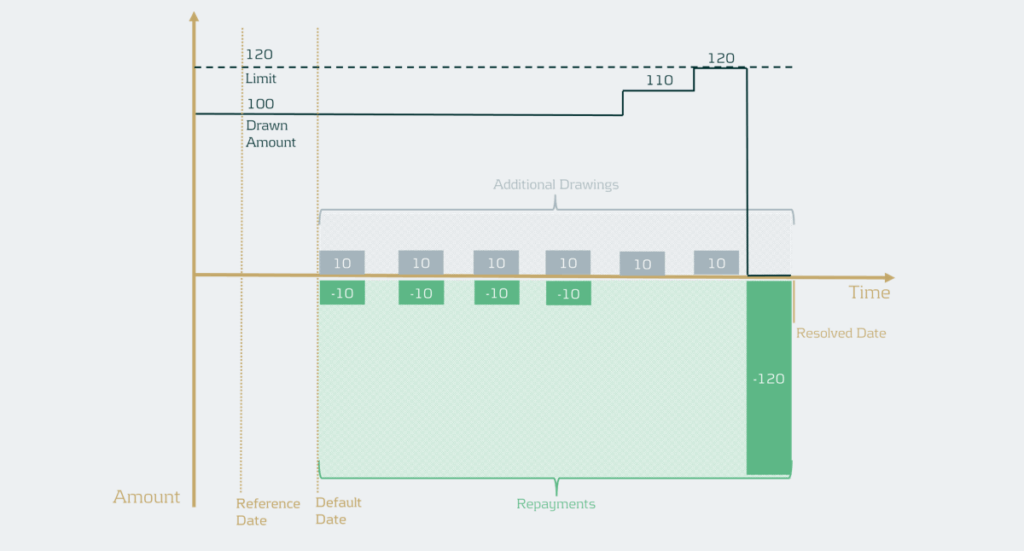
To address this, institutions should now calculate the realized CCF by increasing the drawn amount at default by the positive difference between the highest drawn amount after default and the drawn amount at default. Then the CCF would be (drawn amount at default + additional drawings during default – drawn amount at the reference date) / (limit at reference date – drawn amount at reference date). In the example, the facility has EUR 100 drawn and EUR 20 undrawn at default (and at the reference date for simplicity). The highest drawn amount during default is EUR 120, meaning EUR 20 of additional drawings instead of EUR 60 in the example. Ignoring discounting, this gives a CCF of ((100 + 20) – 100 ) / (120 – 100) =100%. This method uses outstanding balances rather than transaction-level data. It therefore differs from the transaction-based approach typically used in LGD modeling¹. The drawn amounts used in the realized CCF and realized LGD should be consistent, meaning that if an institution currently applies a different method, the LGD model may need to be redeveloped.

Representativeness

While earlier guidelines placed heavy emphasis on ensuring representativeness in the development phase, the proposed guideline focusses on how well the model performs in terms of discriminatory power and homogeneity in rating grades or pools.

However, representativeness remains essential for the data used for developing, testing, and quantifying the CCF models, meaning institutions must still confirm that the data used reflects the characteristics of the application portfolio across different time periods, jurisdictions, and data sources. If the development or testing samples are not representative and this negatively affects model performance or its assessment, they must be redeveloped or adjusted. For the quantification sample, institutions should assess whether any lack of representativeness introduces bias in realized CCFs and apply appropriate adjustments or margins of conservatism where needed, without lowering CCF estimates. Compared to the previous Guidelines on PD and LGD estimation, the new guidelines therefore introduce a simpler approach focused on the performance of the model.

Risk Quantification

Under the EGIM framework, CCF quantification depends on whether the historical observation period is representative of the LRA. If it is, institutions should use the arithmetic average of yearly realized CCFs. If not, adjustments are made to account for underrepresentation or overrepresentation of bad years. The proposed guidelines, however, require a single arithmetic average of all realized CCFs weighted by the number of facilities. It is no longer allowed to use averages based on a subset of observations such as yearly averages. Therefore, potential recalibration is required.

Downturn

The downturn CCF guideline builds on the principles of downturn LGD estimation but introduces several simplifications. The haircut method is removed, as it is considered unsuitable for CCF estimation. Instead, institutions may apply an extrapolation approach at the overall CCF level to capture the direct link between economic factors and CCFs. When no observed or estimated downturn impact is available, a 15%-point add-on is maintained and the105% LGD-cap is removed. Additionally, institutions may apply downturn components estimated for non-defaulted facilities to defaulted ones, eliminating the need for separate downturn estimation and simplifying implementation.

The clarity provided by the new guideline on this topic supports the simplifications aimed to make the framework more pragmatic.

Conclusion

The EBA’s consultation on the new CCF modeling guidelines introduces notable simplifications compared to the previous framework, aiming to enhance consistency across all IRB parameters. While these changes support greater harmonization in credit risk modeling, they also may carry significant implications for institutions, particularly in the areas of level of modeling, realized CCF determination, and long-run average estimation. Adapting effectively to these developments will be essential for maintaining compliance and ensuring robust risk management practices.

The deadline for institutions to submit feedback to the EBA is next week October 29^th 2025. Zanders therefore encourages institutions to evaluate the potential impact on their modeling practices and share insights based on their practical experience.

Reach out to John de Kroon, Dick de Heus, or Louise Schriemer if you are interested in getting a better understanding of what the proposed guidelines mean for your credit risk portfolio.  

In the Netherlands alone, more than €1.4 billion is spent annually on money laundering prevention, with an additional €1 billion in administrative burdens for companies and individuals¹. These costs highlight not only the scale of the challenge, but also the urgent need for technological solutions, such as AI, that are both effective and efficient.

With the rapid rise of artificial intelligence (AI) and increasingly complex regulatory expectations, the field is changing at an unprecedented pace. Keeping up with new developments demands both the right technology and a solid grasp of its principles to maintain fairness, transparency, and effectiveness.

To explain the new developments and how to effectively integrated those, we’re launching a new blog series on the future of FCP: to explore how organizations can balance innovation with responsibility. We will explore the dive into the most pressing challenges in FCP modeling and show how AI and machine learning are shaping its development. Along the way, we’ll share insights on building trust and reliability in next-generation models, along with practical tips, discussion points, and industry perspectives for those working with these emerging technologies.

What to Expect

Each blog post in this series of 4 will focus on a specific topic that is crucial to the present and future of the FCP domain. The posts will follow the typical lifecycle of model development – starting with the development and concluding with validation:

1. Bias and Fairness: AI models are powerful, but they don’t always treat everyone equally, as seen during the “Toeslagenaffaire” in the Netherlands or COMPAS case in the United States. In high-stakes domains like FCP such consequences can be just as severe. In the rush to make AI models “fair”, many organizations fall into the trap of chasing strict statistical parity at the expense of performance and context. In FCP, this tension is especially acute: regulators push for ever-higher recall, while fairness requirements demand balanced precision across different groups. The result? Conflicting objectives, artificial “levelling down,” and potential compliance risks under GDPR. The conventional bias-mitigation mindset is challenged, where a more mature, context-aware approach to fairness is advocated for.
2. Explainability: AI and ML models go hand in hand with the challenge of explainability. These technologically advanced models are frequently described as black boxes: powerful, yet difficult to interpret In practice, model developers outsource the responsibility for model interpretability to SHAP or similar feature-importance methods – and call the job done. But does this really provide meaningful insight into how a model behaves? In FCP, explainability must go beyond technical metrics; it should focus on the people who use these models every day. The real value of AI in this space often lies in how it supports analysts – helping them interpret alerts, make informed decisions, and justify their actions. This article explores how shifting from model-centric to human-centric explainability can transform AI from a black box into a trusted, collaborative partner in the fight against financial crime.
3. Model Drift and Data Drift: The financial world is always in movement. As technologies evolve and customer behaviour shifts, models built to detect financial crime can quickly become outdated. This article explores the importance of monitoring data drift (changes in input patterns) and modeldrift (changes in the relationships between inputs and outcomes). From building models that can withstand shifting behaviour to setting smart thresholds and review cycles, it highlights how banks can keep their FCP models relevant and reliable.
4. The Model Validation Process: Model validation in FCP has long followed the same framework as credit risk – a framework often characterized by manual, time-consuming, and inflexible processes. With criminals constantly adapting their tactics and regulators becoming ever more demanding, this traditional approach is no longer sustainable. This article explores how generative AI can transform model validation without replacing human expertise. When implemented with care and oversight, AI elevates validators, ensuring their skills are applied where they matter most and keeping FCP programs agile in a rapidly evolving landscape.

By progressing through these topics in order – from identifying risks of bias, to ensuring transparency, to monitoring drift, and finally to examining validation frameworks – a clear narrative is created that links principles to practice. Responsible innovation is not just about ticking boxes on a regulatory checklist, it’s about creating an FCP framework that people can trust. These blogs offer insights and perspectives for making this happen.

Looking Ahead

This series of upcoming blog posts is just the beginning. Each topic opens the door to deeper discussions, case studies, and practical applications. Whether you’re a risk manager, data scientist, compliance officer, or executive, the series provides insights into the challenges and practical approaches that financial institutions can take to address them.

Over the past decade, regulatory expectations on European banks’ ESG frameworks have evolved from voluntary disclosure initiatives to detailed operational requirements. While certain regulations such as CSRD and CSDDD have been watered down as part of the Omnibus Directive, EUs climate goals and Climate Law remain intact. The EBA Guidelines on the management of ESG risks will come into force in January 2026, mandating all but the smallest banks to submit annual plans demonstrating how they will reduce their portfolio emissions in time to meet internal and external targets.

Ironically, amidst a slower-than-expected decarbonization in society in general, and with several American and international banks retreating from their climate commitments (and the ensuing collapse of the Net Zero Banking Alliance), it is European banks that are exposed to the largest compliance and reputational risks.

In our experience, many banks may have underestimated the far-reaching impact of the new Guidelines. Unlike previous regulatory guidance, including ECBs Guide on climate-related and environmental risks, what is now required is the complete integration of ESG risks and targets into banks’ ways of working: risk management, client engagement, operations, pricing, and business strategy.

Below we outline the four areas we think will prove the most challenging for banks to implement.

Key challenges

1. Data availability and processes

Banks are required to have in place a structured data environment to enable assessment of ESG risks, with the explicitly stated aim that most of the data should be sourced at the client- and asset level. The Guidelines list a number of metrics that large institutions must define and monitor, including:

• Financed emissions (Scope 1-3)
• Portfolio metrics of clients that are, or are projected to be, misaligned with emission targets
• A breakdown of portfolios secured by real estate according to the level of energy efficiency
• Metrics related to dependencies and impacts on ecosystem services, in particular water
• Metrics related to ESG-related reputational and legal risks (via the banks’ exposures)

Some of these data are already collected and reported by banks, such as financed emissions. But even those metrics rely largely on proxies and assumptions. Even among PCAF member banks the variation in reported emission intensities is significant - and in many cases inexplicable. For many other metrics the data to construct them is either missing or has not even been defined.

Banks need to accelerate their ESG data strategy and decide, for the short- and medium, which data to collect directly from clients andwhich to source from external providers, and the data gaps for which there are no viable alternatives but to use proxies. In turn, for each of these categories there will be many choices to make with implications for quality, timeliness, and costs. In parallel, but informed by the data strategy, the bank needs to decide on – and invest in - their future data infrastructure, which may take years to realize. One obvious case is the need to connect real estate characteristics, such as LTV, flood exposure, energy rating, and insurance coverage with clients’ financial data as well as outputs from climate scenario models.

2. Models and Methods

The Guidelines require banks to map ESG risk drivers to traditional risk categories and – if they are material - embed the risks in several processes: collateral valuation, ICAAP, stress testing, underwriting, and pricing.

The first step in this exercise is to determine which risk drivers are material, and for which risk types. In the end, for most banks, physical and transition risks stemming from climate change will likely prove the most material for credit risk, but ECBs expectations as to the rigor of the materiality assessment - to substantiate such a conclusion - are increasing. For example, banks need to have methodologies in place to assess how and whether social and governance failures in client firms may result in both financial as well as reputational and legal risks.

Even for key risk drivers such as flood risk, banks face a significant challenge in quantifying how and with which probability this will translate into credit risk. It necessitates a number of assumptions such as the response in real estate prices and insurance costs/availability, as well as government policy and disaster funds, flood protection work, and much more. Limited or absent historical data together with the changing nature of risks related to climate change make this kind of model development very different from traditional risk modeling in banks (such as IRB model) and necessitates new expertise.

And while there are several useful publicly available models, in particular by the Net Greening of the Financial System, there is still a lot of work to be done to adapt those scenarios to individual banks’ portfolios and business models.

3. Client engagement and risk assessment

EBA expects climate and environmental risks to be factored into client selection, due diligence, covenants and pricing based, for a start, on an evaluation of counterparties’ transition readiness and resilience to physical risks. Even for large clients that are reporting under CSRD, a lot of the data required to perform these assessments will have to be collected directly as part of the onboarding process.

Although many banks have separate ESG advisory units that support client executives, these are often there to identify opportunities for sustainable products and loans and are not trained to assess and quantify clients’ risks. In the end, it is client executives and credit committees that must stand over the ESG risk assessment and its impact on credit scores, pricing and loan conditions. To save costs and time for client-facing staff, they should be equipped with practical and user-friendly tools and systems that support them in collecting and organizing relevant ESG data.

Worse, for most SME and retail customers there is no dedicated account manager, the on-boarding and credit process is largely automated. Banks should develop a risk-based sourcing strategy that, at least initially, uses sector-level proxies for the majority of firms while collecting individual data from those that have been designated as high-risk clients. Again, a number of choices have to be made when developing such a framework to ensure it is purposeful.

4. Governance and steering

What we deem most pressing  for banks is to decide on their governance to triage and drive progress on the vast array of requirements. It will require strong leadership and a project committee with sufficient seniority to make crucial, and potentially costly decisions. Elaborate RACIs will be of little use if those assigned ownership are found too low in the bank’s hierarchy.

While the exact division of responsibilities will depend on each bank’s structure and governance model, it is clear that the actual transition plan(s) should be owned by the first line (and subsequently validated by second line), and tie into existing business planning and strategic process.  At the same time, the transition plan will be part of the annual ICAAP submission, which is a second-line responsibility, and the bank’s ESG strategy should be reflected in the business resilience test . Hence, these first- and second-line processes must be aligned.

The Board and CEO should set the bank’s ESG strategy and ensure that these expectations are actionable. Little progress is to be expected if C-suite members do not have clear KPIs and KRIs tied to the delivery of the bank’s transition plan. Quantitative targets may be based on, in addition to financed emissions, the energy efficiency profile of the mortgage book, sustainability-linked bond issuance, and the funding of low-carbon power production. Such targets may necessitate difficult trade-offs, including tighter origination criteria, off-boarding of high-risk clients, and larger discounts for green loans.

Purposeful implementation strategy

To succeed in this potentially daunting endeavour banks should adopt a pragmatic implementation approach, balancing costs against compliance risks. The ECB and local supervisors are fully aware that banks need considerable time to get all prerequisites in place, and the scope and detail of transition plans must be allowed to evolve over years.

However, while early transition plans cannot be expected to present the ultimate answers to either data, methodological or governance challenges, , banks should be able to demonstrate their capacity to achieve essential climate and environmental objectives. Quantitative targets, in particular regarding a bank’s financed emissions, must be achievable.

Finally, underscored by recent legal cases, any claims related to the bank’s “green” credentials must be based on evidence. The heightened compliance and legal risks mean that it is timely to review the bank’s public as well as non-public ESG commitments, benchmark them against peers, and make an honest assessment of the costs and resources necessary to fulfil them.

Want to find out more about how Zanders can assist your bank in developing your ESG strategy and meet regulatory expectations?

Reach out to our Partner Lars Frisell, our ESG and risk management expert, for tailored guidance.

November 2025 marks the end of the Swift MT-MX co-existence phase, which will see the adoption of ISO 20022 XML messaging in the interbank space for cross border payments. Whilst this Swift migration represents possibly the most significant disruption to traditional global cross border payments since Swift first introduced electronic financial messaging back in 1977, ultimately this is just a message format change, which still fails to address some of the key challenges around cross border payments. In this latest article from Eliane Eysackers and Mark Sutton, they provide a recap on the remaining challenges with cross border payments in addition to focusing on the rapidly evolving payments landscape, which will redefine what is possible.  

Background

Whilst the evolution of the payments industry over the past twenty years has been significant, both in terms of the number of available payment methods and how payments can now be made, the intensity of focus increased significantly when the G20 endorsed the Roadmap for Enhancing Cross-border Payments¹ in 2020. The G20 made enhancing cross-border payments a priority – specifically making cross-border payments, including remittances, faster, cheaper, more transparent and inclusive.

Friction will remain with the legacy Correspondent Banking Model

Post the Swift MT-MX migration, the correspondent banking model will remain an essential part of the cross border payments flows. Underpinned through a foundation of bilateral agency agreements, whereby one bank maintains a physical bank account (and deposits) with another (correspondent) bank, corporate treasury will continue to experience friction in the following areas:

High Costs	The cost of a cross-border wire payment extends beyond the charges of the originating bank. Under the correspondent banking model, each bank involved in the cross-border payment processing chain can apply a fee, including the beneficiary bank.
Slow Processing	Whilst Swift GPI is a significant enhancement that provides tracking of the cross-border payment status, this merely highlights that in some cases, a cross border payment can still take 24 hours to reach the beneficiary bank account.
Principle Amount	Whilst the Swift message design allows for the originating customer to specify if the beneficiary should receive the full principle (payment) amount, a significant number of corporates still encounter challenges where at least one bank in the payment chain deducts their fees from the principal payment amount. This means the beneficiary receives less money, creating reconciliation challenges and customer dissatisfaction.
Settlement Risks	Banks worldwide need to hold significant balances in reserve to cover the risk of correspondent bank default because many cross-border payments take a day or more – sometimes weeks – to complete.  CLS, which was launched in 2002 to mitigate this risk, only covers a small number of the world’s currencies, leaving large sectors of the global economy badly exposed to correspondent banking’s overnight risk problem

The Digitization of Money – Taking Cross Border Payments to the Next Level

The race is now on as the rapid evolution of technology provides the opportunity for greater speed, transparency and efficiency within the cross-border payments domain. There are a number of projects at different stages of maturity that leverage distributed ledger technology to support the digitisation of cross border transactions:

• BIS Project m-Bridge (2021-2024)

Originally launched by the Bank for International Settlements (BIS) in collaboration with the central banks of China, Hong Kong, and the United Arab Emirates, this project aimed to create a multi-central bank digital currency (m-CBDC) platform that addressed key inefficiencies in cross-border payments, including high costs, low speed and operational complexities. Furthermore, this platform would be fully compliant with jurisdiction-specific policy and legal requirements. However, the 2024 BRICS summit also included Egypt, Ethiopia, Iran, and the United Arab Emirates as members², with the agenda including a discussion around the creation of a BRICS Bridge which would be based on m-bridge technology. Recognising that a BRICS Bridge offered the potential for some independence against US supervised financial systems and the current restrictions to Swift, the BIS announced in October 2024 that mBridge had reached the minimum viable product (MVP) stage in mid-2024 and that it was now handing over to the participating central banks to carry the project forward.  

With the technology proven and China at the helm, we are now hearing some news about Chinese banks executing cross border payments using mBridge³. We should expect transactional volumes to increase through 2025 and assuming this project is viewed as a success, an expansion across parts of Asia and possibly the Middle East Region given the participating central banks⁴.

• Project Agorá (2024 - now)

Commencing in April 2024, Project Agorá is the BIS Innovation Hub’s largest and most complex project in geographical scope and number of participants. The project’s main objective is to demonstrate how a unified ledger could enhance the efficiency of business and regulatory processes in correspondent banking payment chains, thereby reducing transaction times and costs, enhancing payment transparency, and mitigating risks for banks involved in cross-border payments.

The project aims to build a technical prototype to test wholesale cross-border payments to demonstrate the following:

1. The ability to represent tokenised commercial and wholesale central bank money on a unified ledger that meets technical and business requirements.
2. Atomic cross-border transactions between currency areas leveraging a single currency pair or a vehicle currency in a way that preserves depositor-bank relationships.
3. The ability to streamline pre-validation efforts, e.g. reducing duplication of efforts, in the payment chain without changing existing standards and requirements.
4. Improved efficiencies in complying with sanctions screening as well as anti-money laundering and rules on countering the financing of terrorism.

This project brings together seven central banks⁵ which will work in partnership with 42 financial services companies⁶ and convened by the Institute of International Finance (IIF)⁷. Project Agorá aims to go beyond proof of concept and deliver a prototype to test a range of potential current and future use cases. The lessons learned during the project may set out a path for a new type of financial market infrastructure tailored to cross-border payments based on new technology.

The project is currently in its final design phase, which will then allow the BIS to issue an RFP to choose a technology partner. A project report is expected to be published by the end of 2025.

• Partior (2021 - now)

Singapore based Partior is a blockchain-based fintech, which is offering a next-generation atomic settlement network for cross-border wholesale payments. Founded in 2021, it was announced as the winner of the 2022, G20 Indonesia Techsprint challenge on CBDCs. Backed by DBS Bank, J.P. Morgan, Standard Chartered, Temasek, and Peak XV, it processed over USD 1 billion in transaction value in November 2024⁸, marking a significant milestone in the company's journey to deliver instant cross-border transactions for financial institutions.

Banks either using or partnering with Partior include its founders DBS Bank, JP Morgan, and Standard Chartered, along with Deutsche Bank, Emirates NBD, and Nonghyup Bank, who are using it to facilitate real-time, cross-border payments and settlement, often involving tokenized commercial bank money to address inefficiencies like settlement delays, limited transparency, and high operating costs in the global financial market by removing intermediaries.

Whilst Partior's platform currently supports USD, EUR, and SGD, there are plans to integrate additional currencies combined with expanding its network across the Americas, EMEA, and Asia.

• Regulated Liability Network (2021 - now)

With origins dating back to the 2021 Monetary Authority of Singapore (MAS) global CBDC solutions challenge, the evolution continued in 2024 with UK Finance announcing work on a new UK Regulated Liability Network (RLN) experimentation phase with eleven of its members⁹. This was completed during Q3 2024 and explored the possible benefits of tokenisation, distributed ledger technology (DLT), and programmable money.

The focus earlier this year was on the technology build, test, and delivery for a pilot phase. Developing the technology framework included the orchestration layer, associated tokenised deposit and shared ledger systems. The objective is to build a regulated financial market infrastructure using distributed ledger technology (DLT) to enable new digitised payment and settlement capabilities. In September 2025, UK Finance issued a press release¹⁰ confirming a pilot will run until mid-2026 with the objective of demonstrating tangible benefits to customers, businesses and the wider UK economy.

• J.P. Morgan launches USD Deposit Token, JPMD (June 2025)

In addition to the various industry collaborations, we are also seeing commercial banks developing solutions that will address the current friction in the cross-border payments space as well as enhancing existing payment capabilities. J.P. Morgan introduced the JPMD deposit token in a proof-of-concept launch on the ^{24th of} June, 2025, on the Base public blockchain, developed by Coinbase¹¹. The JPMD token serves as a digital representation of commercial bank money and is an alternative to stablecoins for J.P. Morgan's institutional clients. Whilst Deposit Tokens and stablecoins can be applied to similar use cases, Deposit Tokens differ from stablecoins in key areas including, interest payouts, and deposit treatment.

What are the Benefits of Digitized Cross Border Payments?

Harnessing new digitised cross border payment rails that are underpinned with distributed ledger technology and smart contracts will address the legacy frictions arising from the separation of messaging, clearing and settlement. Benefits include the following:

• Atomic settlement: Has emerged with the advent of blockchain technology and distributed ledger systems. Whilst the legacy settlement processes often involves multiple intermediaries and can take days to complete - which expose participants to counterparty and settlement risks, atomic settlement enables instant and simultaneous completion of a series of transactions, ensuring instant and irrevocable value transfers, importantly eliminating settlement risk.

• Faster processing speed: Industry analysis of Swift versus RippleNet highlighted RippleNet settles payments in 3–5 seconds using XRP, while Swift can takes days due to the use of intermediaries. Swift only handles messaging; the actual fund movement depends on multiple banks and currencies.

• Reduced cost: Fewer intermediaries are involved in the cross-border payment processing chain.  

Lastly, these new digitised payment rails will support programmable payments, enabling the contingent performance of actions through smart contracts, for example only release payment when the goods have been received.  

Conclusion

The world is witnessing significant growth in cross-border payments, which has been driven by the globalization of trade, capital and migration flows. Global payments are expected to increase from USD 190 trillion in 2023 to USD 290 trillion by 2030¹². Streamlining international transactions by reducing settlement times, certainty, cost and risk is now becoming a strategic imperative.

However, the above selected projects represent just a few of the initiatives underway at the moment as the digital payments landscape continues to evolve. Whilst it does look like a fragmented digital payments landscape will be the ultimate outcome, what is clear is that programmable payments and smart contracts can enable new ways of atomic settlement, unlocking new value-added solutions that are simply not possible or practical under current payment rails. These new digital payment rails will eliminate the legacy inefficiencies that exist today with cross border payments, reducing costs, and providing atomic settlement. The future of cross border payments is now looking faster and smarter.