Whilst embarking on a digital transformation journey will bring operational and financial efficiencies, it also expands the attack surface and introduces new vulnerabilities, which allow cyber criminals and bad actors to operate with greater sophistication and speed.

Current projections indicate that global Authorized Push Payment (APP) fraud losses could reach US$331bn by 2027¹. In the US alone, the FBI's IC3 reported over 859,00 complaints in 2024, with $16.6 billion in losses. Phishing and social engineering dominate as entry vectors, but compromised credentials are becoming more common with approximately 22% of breaches now starting with stolen login data². Finally, the average cost of ransomware recovery in 2024 reached $2.73 million, with an average of 21 days of downtime for organizations.

These are concerning numbers and in this joint article Mark Sutton (Zanders) and Andrew Compton (Cortida) highlight some of the key risks within both the systems landscape and the underlying operational processes and provide some suggestions around possible risk mitigation.

What are the Key Risks

The current cybercrime and payment-fraud risk landscape is being shaped by four foundational forces linked to:

• The rise of the digital agenda, including instant payments within corporate treasury,
• The darker side of AI which is enabling fraud,
• The increase in professionalized cybercrime,
• and lastly, an increasingly interconnected and complex ecosystem.

As the above foundational forces converge, we see the manifestation in corporate treasury through various risk categories (including but not limited to):

• Business email compromise (BEC) and impersonation fraud.
• AI-enabled social engineering and identity fraud.
• Real-time payment fraud risk.
• Vendor / supplier payment fraud and master-data compromise.
• Malware and ransomware.
• Supply-chain compromise.

Possible Risk Mitigation Options

Practical mitigation options are based on a combination of process, technology and governance measures that must:

• Include a strategy that removes the reliance on email or voice as a trusted payment instruction channel.
• Require design controls that assume identity signals can be spoofed.
• Accelerate fraud detection to before payment release rather than after.
• Elevate controls to protect vendor master data as a critical financial asset.
• Ensure treasury and payments endpoints are recognised as critical payment infrastructure.
• Extend treasury control framework beyond organizational boundaries.

How can Zanders/Cortida Help?

Corporate treasurers now need to move away from a reactive approach to an "always-on" monitoring, control and mitigation operating model. Effective risk mitigation now requires a layered control model that combines process, technology, governance, and behavioural controls. The Zanders/Cortida partnership considers the full end-to-end payment risks landscape through a structured payment and systems security framework.

If you would like to learn more about this new service, please speak to your Zanders relationship contact to arrange a more focused discussion.

This article was first published on: TMI (Treasury Management International).

Cross-border payments remain one of the last great friction points in global finance. Despite decades of incremental improvement, corporate treasurers at the world's largest companies still contend with settlement delays measured in days, opaque fee structures, and an architecture that separates messaging from settlement in ways that create cost, risk and operational complexity.

This is not a new observation. The G20 made enhancing cross-border payments a priority in 2020¹, and every major industry body has published recommendations since. What is new is that a credible alternative infrastructure now exists; not in theory, but in production. Stablecoin-based settlement rails, underpinned by distributed ledger technology and institutional-grade custody, are moving from proof of concept to live deployment.

This article examines why the current correspondent banking model creates persistent friction, how stablecoin settlement infrastructure addresses each pain point, and what this means for corporate treasury teams preparing for the next generation of payment rails.

The Correspondent Banking Model: Persistent Friction at Scale

The architecture of cross-border payments has remained fundamentally unchanged for decades. When a corporate treasurer in London needs to pay a supplier in Singapore, the payment traverses a chain of correspondent banks, each maintaining bilateral relationships, each potentially applying fees, each adding processing time.

This model creates four categories of friction that corporate treasury teams manage daily:

1. Cost Accumulation

Each bank in the cross-border chain can apply fees, including intermediary and beneficiary banks. For multinationals managing thousands of payments monthly, these costs compound into millions annually.

2. Settlement Latency

Swift GPI² improved visibility through payment tracking, but tracking a slow payment does not make it faster. Cross-border payments routinely take 24 to 48 hours to reach the beneficiary.

3. Principal Integrity

Intermediary banks frequently deduct fees from the payment itself. The supplier receives less than invoiced, triggering reconciliation queries and damaged supplier relationships.

4. Settlement Risk

CLS³ Bank covers only 18 currencies, leaving large swathes of global trade exposed to overnight and multi-day settlement risk in the correspondent banking model.

These are not edge cases. They are structural features of the correspondent banking model, experienced daily by every corporate treasury function operating internationally.

It is worth emphasizing that this is not a criticism of the banks and institutions that operate within the correspondent banking framework. These institutions have invested heavily in modernization; the Swift MT to MX migration⁴, GPI tracking, pre-validation services. These investments have delivered genuine improvements. The point is structural: the separation of messaging from settlement, the reliance on chains of bilateral banking relationships, and the batch-processing cadence of traditional payment systems create inherent limitations that no amount of incremental optimization can fully resolve.

Stablecoin Settlement: A New Architecture

Stablecoin-based payment infrastructure does not incrementally improve the correspondent banking model. It replaces the underlying architecture with one designed for the requirements of modern treasury operations.

Atomic Settlement

The transfer of value and its confirmation occur in a single, indivisible operation. Settlement finality is measured in seconds, not days. Settlement risk is eliminated entirely.

Continuous Operations

24 hours a day, 365 days a year. No cut-off times, no batch processing windows, no weekend closures. Genuine real-time liquidity management across every time zone.

Transparent Costs

Visible, predictable fee structures with no hidden intermediary charges. The sender knows the cost upfront; the beneficiary receives the full amount.

Programmability

Smart contracts enable conditional payments, automated sweeps, threshold-triggered distributions and rules-based treasury operations as native capabilities.

Programmability transforms payment operations from a sequence of manual instructions into an automated, rules-based system. The implications for cash management, working capital optimisation and supply chain finance are substantial.

The Institutional Infrastructure Is Ready

A common objection, particularly from risk-conscious treasury functions, has been that stablecoin infrastructure lacks the institutional controls required for corporate use. This objection was valid two years ago. It is no longer accurate.

Regulated instruments. MiCA⁵ in Europe and emerging frameworks in the US, Singapore and the UAE have created regulatory clarity for stablecoin issuance, reserve management and redemption. Corporate treasurers can now evaluate stablecoins within established regulatory frameworks rather than operating in a legal grey area.

Institutional custody. Qualified custodians now offer segregated custody, insurance coverage and the maker-checker controls that corporate treasury functions require. The custody infrastructure for digital assets has converged with the operational standards of traditional securities custody.

Settlement venues. Institutional-grade settlement venues provide the compliance, onboarding and operational frameworks that connect regulated financial institutions with stablecoin infrastructure. These are not experimental platforms; they are production environments designed for institutional throughput.

Network diversity. Corporate treasurers are not limited to a single blockchain network or a single type of digital money. The toolkit now spans regulated stablecoins, tokenized bank deposits, and tokenized money market funds; providing the diversification across risk, yield and liquidity dimensions that prudent treasury management requires.

What This Means for Corporate Treasury

The practical implications for corporate treasury teams are significant and near-term:

• Working capital release

Reducing settlement times from days to seconds releases trapped liquidity across the payment cycle. For a multinational with billions in transit, even a one-day reduction can release hundreds of millions in working capital.

• Operational simplification

Programmable payments reduce manual intervention for conditional payments, multi-currency sweeps and intercompany settlements. More automated, more auditable, less error-prone.

• Risk reduction

Atomic settlement eliminates counterparty exposure inherent in multi-day settlement windows. Capital currently reserved against settlement risk can be redeployed.

• Cost reduction

Fewer intermediaries, transparent fee structures and automated processing reduce the total cost of cross-border payment operations.

• New capabilities

Automated liquidity rebalancing, conditional supply chain payments, real-time cash concentration across entities and jurisdictions; strategies simply not possible on current rails.

The Transition Has Begun

Global cross-border payment flows are projected to grow from $190 trillion in 2023 to $290 trillion by 2030⁶. The infrastructure that processes these flows will determine the cost, speed and risk profile of international commerce for the next decade.

The correspondent banking model served global trade well for half a century. But the structural separation of messaging from settlement, the reliance on chains of bilateral relationships, and the batch-processing architecture of legacy systems create friction that incremental improvement cannot fully resolve.

Stablecoin settlement infrastructure offers a genuine architectural alternative; one that delivers atomic settlement, continuous operations, cost transparency and programmability. The regulatory frameworks are in place. The institutional infrastructure is ready. The instruments exist.

For corporate treasury teams, the question is no longer whether stablecoin-based settlement will play a role in cross-border payments. It is how quickly to develop the internal capabilities, governance frameworks and banking relationships needed to access these new rails.

The transition has begun. The treasurers and institutions that engage now will shape the standards. Those that wait will adopt them.

What treasurers should do to prepare

Identify the use cases based on high-friction corridors (for example, cross-border payments to emerging markets or intercompany funding) where traditional payment rails struggle. This process will highlight both the business need and potential urgency around experimentation.

The next step is to engage in more detailed conversations with possible partners and vendors to determine any key dependencies, critical actions and potential timelines. This detailed analysis will help treasury take the transformational step from being a passive observer to an active participant in the new, real-time digital financial landscape.

Executive Summary

RMA will be an optional model within IFRS 9 for net interest rate repricing risk¹ in dynamic, open portfolios (for example, where new deposits or loans are continually added and existing positions mature or reprice). The IASB also proposes withdrawing the IAS 39 macro hedge requirements (and the IFRS 9 option to apply them) and adding related IFRS 7 disclosures.

Compared with current IFRS 9 hedge accounting, RMA shifts from item-level hedges to portfolio net-position accounting, better aligned to typical banking book features (for example, non-maturity deposits and pipeline exposures). Compared with IAS 39 macro hedging (including the EU carve-out), it replaces bucket-based rules and carve-out reliefs with a principles-based net exposure model.

At a high level, the RMA model works as follows:

• Set the target: the entity specifies how much net interest rate risk it aims to mitigate over time, within defined risk limits and not exceeding the net exposure in each time band (bucket). The target can be updated prospectively as the balance sheet evolves.
• Link to derivatives: external interest rate derivatives can be designated. The model uses benchmark derivatives (hypothetical instruments with zero fair value at inception) to represent the risk the entity intends to mitigate.
• Recognize an adjustment: a risk mitigation adjustment is recognized on the balance sheet. It equals the lower of (I) the cumulative value change of the designated derivatives and (II) the cumulative value change of the benchmark derivatives. Any remaining derivative gains or losses (and any ‘excess’ adjustment) go to profit or loss.
• Release to earnings: the risk mitigation adjustment is released to profit or loss as the underlying repricing effects occur.

RMA is a meaningful step toward aligning accounting with how banks manage banking-book interest rate risk in dynamic, open portfolios. At the same time, the ED leaves important practical questions open, notably on benchmark-derivative construction, operation of the excess test, and the level of data, systems, and governance needed for ongoing application.

After the 31 July 2026 deadline, the IASB will review comment letters and fieldwork feedback and decide whether further deliberations are needed, so finalization is likely to take several years. Even once the IASB issues a final standard, application in the EU would still depend on completion of the endorsement process (EFRAG advice, Commission adoption, and Parliament/Council scrutiny).

Introduction

On December 3^rd, 2025, the IASB published the ED proposing RMA for interest rate risk in dynamic portfolios. RMA is the result of the IASB’s long-running efforts on accounting for dynamic interest rate risk management, previously referred to as DRM. RMA focuses on repricing risk, which is the interest rate risk that arises when the timing and amount of repricing differ between assets and liabilities.

The aim is to better reflect how banks manage interest rate risk in the banking book at a portfolio level, an area where existing hedge accounting requirements have long been seen as difficult to apply in a way that aligns with real-world balance sheet management.

The IASB presents RMA as a step forward, to better reflect how banks manage interest rate risk in the banking book at a portfolio level, an area in which existing IAS 39 and IFRS 9 hedge accounting requirements have long been viewed as difficult to apply in a way that aligns with real-world, dynamic balance sheet management. In the IASB’s view, RMA is intended to improve that alignment, increase transparency about the effects of repricing-risk management on future cash flows, strengthen consistency between what is managed and what is eligible for accounting treatment, and recognize in the financial statements the extent to which repricing risk has actually been mitigated and the related economic effects.

This article provides a structured overview of the proposed RMA model and its key mechanics. Throughout the article, Zanders provides practical insights on the impact on entities, highlighting the key areas that will shape implementation challenges and accounting results. These insights draw on Zanders' 2025 survey on interest rate risk management and hedge accounting, as well as analysis of stakeholder feedback such as EFRAG's draft comment letter². The practical implications will depend in part on the outcome of field testing.

Overview of RMA

The model components and their relationships are presented in Figure 1 below:

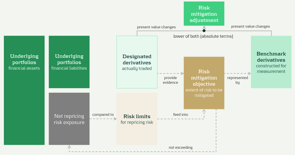
Figure 1: RMA model component overview (source: IASB ED – Snapshot, December 2025)

The RMA model is built around a small set of linked building blocks that start with the bank’s balance-sheet exposures and end with the accounting adjustment that reflects risk management in the financial statements:

• Underlying portfolios: the managed portfolios that expose the entity to repricing risk.
• Net repricing risk exposure: the net position created by the interaction of asset and liability repricing profiles (i.e., the aggregate repricing mismatch the bank is exposed to).
• Risk limits: the bank’s risk appetite and constraints for the managed exposure. In the model, these limits act as an important boundary.
• Risk mitigation objective: the clearly articulated target for how much of the net repricing risk exposure management intends to mitigate (within risk limits). This objective is the central anchor in the model.
• Designated derivatives: the derivatives the bank trades to achieve the risk mitigation objective.
• Benchmark derivatives: hypothetical derivatives constructed to represent the risk mitigation objective for measurement purposes. They translate the objective into a measurable reference profile against which fair value changes can be assessed.
• Risk mitigation adjustment: the accounting output of the model, which is the lower of the change in fair value of the benchmark derivatives and the designated derivatives (in absolute terms).

The section headers contain the relevant paragraph of the ED. The body of the text refers to the ED amendments to IFRS 9 [7.x.), application guidance [B7.x.x), basis for conclusions [BCx), and illustrative examples [IEx), and amendments to IFRS 7 [30x).

Speak to a Zanders expert

Objective and scope [ED 7.1]

IFRS 9 hedge accounting improves alignment for many strategies, but it does not fully capture dynamic, open-portfolio (macro) management of banking book repricing risk—where entities manage interest rate risk of net open positions rather than hedging individual instruments. The RMA model is intended to reflect this more directly and reduce reliance on proxy hedges that can obscure transparency and comparability.

The objective and scope of RMA can be summarized as follows:

• Objective: RMA is, like current hedge accounting under IAS 39 and IFRS 9, an optional model within IFRS 9. The objective is to reflect the economic effect of risk management activities and improve transparency by explaining why and how derivatives are used to mitigate repricing risk and how effectively they do so —bringing reporting closer to actual interest rate risk management practices [7.1.3]. It is the IASB’s intention to withdraw the requirements in IAS 39 for macro hedge accounting and the option in paragraph 6.1.3 of IFRS 9 to apply the requirements in IAS 39 to a portfolio hedge of interest rate risk.
• Scope/eligibility: An entity may apply RMA if, and only if, all of the following are met [7.1.4]:
  • Business activities give rise to repricing risk through the recognition and derecognition of financial instruments that expose the entity to repricing risk.The risk management strategy specifies risk limits within which repricing risk, based on a mitigated rate, is to be mitigated, including the time bands and frequency.
  • The entity mitigates repricing risk arising from underlying portfolios on a net basis using derivatives, consistent with the entity’s risk management strategy.
• Application discipline: RMA is applied at the level where repricing risk is actually managed and requires robust formal documentation (strategy, mitigated rate, mitigated time horizon, risk limits, and methods for determining exposures and benchmark derivatives) [7.1.6, 7.1.7].

Key considerations and insights

1. Objective: RMA’s objective to reflect the economic effect of risk management activities may not always coincide with eliminating accounting mismatches (as suggested by other key considerations and insights later in this article). For example, EFRAG’s draft comment letter agrees that faithful representation is a key objective and could improve current accounting, for example, by reducing reliance on proxy hedging. However, it questions whether this should be treated as equally important as eliminating accounting mismatches. This aligns with the concerns expressed around the impact on the hedge effectiveness by several European banks in Zanders’ 2025 survey on interest rate risk management and hedge accounting3, while more than 80% of the participants assessed its effectiveness under the current hedge accounting approach as acceptable.

Net repricing risk exposure [ED 7.2]

Entities are required to determine a net repricing risk exposure across underlying portfolios by aggregating repricing risk exposure using expected repricing dates, within each repricing time band as required to be defined in formal documentation.

Key requirements include:

• Eligible items Underlying portfolios can include [7.2.1; B7.2.1–B7.2.2]:
  • Financial assets measured at amortized cost or FVOCI,
  • Financial liabilities at amortized cost, and,
  • Eligible future transactions that may result in recognition/derecognition of such items.
• Portfolio view and behavioral profiles: Items that may not show sensitivity on an individual basis (for example, demand deposits) can still contribute to repricing risk on a portfolio basis. A stable ‘core’ portion may be treated as behaving like longer-term funding if supported by reasonable and supportable assumptions and consistent with risk management [B7.2.2].
• Expected repricing dates and time bands: Expected repricing dates must be measured reliably using reasonable and supportable information (including behavioral characteristics such as prepayments and deposit stability). Time bands and risk measures (e.g., maturity gap or PV01) must be consistent with actual risk management [7.2.5–7.2.9; B7.2.10–B7.2.16].
• Equity modeling as a proxy: Own equity is not eligible for inclusion in underlying portfolios, but the model acknowledges that some entities assess repricing risk from cash/highly liquid variable-rate assets only to the extent they are ‘funded by equity’. If internal equity modeling (e.g., replicating portfolios) is used for risk management, it can serve as a proxy to determine how much of those exposures are included in net repricing risk exposure [B7.2.17; IE184-IE191].

Key considerations and insights

2. Eligibility: RMA aims to reflect net repricing risk management, but eligibility rules can make the net repricing risk exposure only a partial proxy for the position Treasury actually manages. For example, banks might include fair value through profit or loss (FVTPL) items for interest rate risk management but these are not allowed as underlying items in the net repricing risk exposure (also noted by EFRAG).

3. Risk management by time bands (1/2): RMA requires a risk mitigation objective based on the net repricing risk exposure determined for each repricing time band, but it is unclear how entities that do not manage their interest rate risk across time bands would then apply the RMA model, as noted by EFRAG.

4. Risk management by time bands (1/2): RMA requires the same risk measure (e.g., maturity gap or PV01) for all exposures within each repricing time band [B7.2.13], but banks’ risk management practice might deviate from this.

5. Equity treatment: RMA introduces an equity proxy approach that allows partial inclusion of variable-rate assets based on modelled equity, viewing equity as residual and ineligible for direct inclusion. This is an addition compared to the DRM staff papers. Banks' risk management practices might treat equity differently (e.g., by modeling it).

Designated derivatives [ED 7.3]

Under RMA, banks can designate external derivatives (e.g., interest rate swaps, forwards, futures, options) used to manage net repricing risk as hedging instruments. Eligible derivatives are generally consistent with IFRS 9. All designated derivatives collectively mitigate the net portfolio risk and remain recognized at fair value.

Eligibility depends on the following items:

• Mitigation: Derivatives can only be designated to the extent that they mitigate the net repricing risk exposure [7.3.6].
• External counterparty: Derivatives must be with a counterparty external to the reporting entity. Intragroup derivatives may qualify only in the separate or individual financial statements of the relevant entities, and are not eligible in the consolidated financial statements of the group [7.3.4].
• Designate once: Derivatives already in a hedging relationship for interest rate risk in accordance with Chapter 6 of IFRS 9 are not eligible [7.3.5].
• Options: Written options are generally excluded, unless part of a net written option position that offsets a purchased option, resulting in a net purchased position overall [7.3.2(a), 7.3.3].

Banks can designate derivatives in full or in part (e.g., designating 80% of a swap if only that portion manages interest rate risk), but the selected portion must align with the documented risk mitigation objective.

Once derivatives are designated, they can only be removed from RMA if they are no longer held to mitigate the net repricing risk exposure under the entity’s risk management strategy.

Key considerations and insights

As the EFRAG comment letter notes: 6. Options and off-market derivatives: Further guidance is needed on how to treat options (for example, time value) and off-market derivatives (non-zero initial fair value) within the designation mechanics.

7. De-designation: The ED does not allow voluntary de-designation, but banks often manage changes by entering into offsetting trades rather than settling existing positions.

Risk mitigation objective [ED 7.4]

The risk mitigation objective is the bridge between risk mitigation intent and what’s actually executed: it sets how much net repricing risk exposure the entity aims to mitigate within risk limits [7.4.2]. The benchmark derivatives and consequently the risk mitigation adjustment are built from this risk mitigation objective (see next sections), enabling partial hedging while avoiding objectives that aren’t supported by actual designated hedges. [ED 7.4.1, B7.4.2–B7.4.3].

Key requirements:

• Evidence-based: The objective must be consistent with the repricing risk mitigated by designated derivatives—it’s a matter of fact, not a free choice. [ED 7.4.1, B7.4.2–B7.4.3]
• Absolute, not proportional: It’s stated as an absolute amount of risk (e.g., PV01), not ‘X% of each instrument’ [B7.4.2].
• Capped by exposure: It cannot exceed net repricing risk exposure (overhedge) in any time band [7.4.1, B7.4.2–B7.4.3].
• Measurement basis: The risk mitigation objective should be set using the same risk measure (e.g., DV01) used to quantify exposure [ED B7.4.1].

Key considerations and insights

8. Repricing time bands are a key design choice: the risk mitigation objective is specified and capped by the net repricing risk exposure in each time band. Executing (and designating) hedges in neighboring tenors (a common practice) can create residual P&L volatility, because only the portion aligned to that time band’s net repricing risk exposure is reflected in the risk mitigation adjustment.

9. Degree of freedom risk limits: While RMA imposes strict alignment requirements between net repricing risk exposure, risk mitigation objective, and designated derivatives on measures and time bands, entities retain strategic flexibility on risk limits. Risk limits do not need to be specified per time band [B7.4.6], allowing entities to set overarching frameworks rather than granular constraints.

Benchmark derivatives [ED 7.4]

Benchmark derivatives are introduced to measure hedge performance: modelled (hypothetical) derivatives that are not executed and not recognized on the balance sheet, but are constructed to replicate the timing and amount of repricing risk captured in the risk mitigation objective, as presented in Figure 1 above and Figure 2 below.

In practice, the benchmark derivative is designed to mirror the bank’s target risk position (e.g., a swap profile that matches the repricing ‘gap’ being mitigated), so its fair value movement represents how the net repricing risk exposure would change when interest rates move. If an entity intends to mitigate 70 of the 100 units of repricing risk in the 9-year time band by a 10-year swap, the benchmark derivative is based on 70 units and 9 year maturity [B7.4.8].

Benchmark derivatives should have an initial fair value of zero based on the mitigated rate [7.4.5]. These benchmark derivatives are therefore similar to the hypothetical derivative used in cash flow hedging [B6.5.5–B6.5.6 of IFRS 9].

Key considerations and insights

10. Operational burden (1/3) – benchmark derivatives: RMA intentionally separates designated derivatives from benchmark derivatives (constructed to start at zero fair value at the mitigated rate), so they won’t always share the same terms. This can become operationally heavy, as also noted by EFRAG.

Risk mitigation adjustment [ED 7.4]

The risk mitigation adjustment is the accounting output of the model and is presented as a single line item on the balance sheet (asset or liability). At each reporting date (so not necessarily the hedging date), the entity compares the cumulative fair value change of all designated derivatives with the cumulative fair value change of all the benchmark derivatives, and recognizes the lower of those two amounts (in absolute terms) [7.4.8] as the risk mitigation adjustment. That balance sheet adjustment is the mechanism that offsets the designated derivatives’ fair value changes in profit or loss; any remaining gain or loss (i.e., the portion not captured by the lower-of) is recognized directly in profit or loss as residual volatility/ineffectiveness [7.4.9].  This is visualized in Figure 2 below.

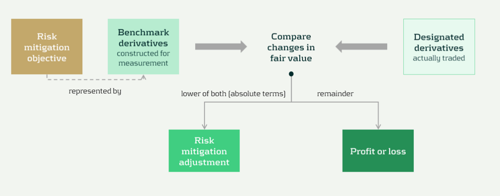
Figure 2 Recognition and measurement of risk mitigation adjustment (source: IASB ED – Snapshot, December 2025)

The 'lower of' mechanism ensures the risk mitigation adjustment never exceeds what's actually supported by either (I) the designated derivatives or (ii) the net exposure being hedged. This prevents over-recognition of hedging effects.

The risk mitigation adjustment is then recognized in profit or loss over time on a systematic basis that follows the repricing profile of the underlying portfolios [7.4.10], so the hedging effect shows up in the same periods in which the hedged repricing differences affect earnings.

Key considerations and insights

11. Operational burden (2/3) – risk mitigation adjustment: Heavy tracking requirements (including effects of settling vs offsetting trades), unclear calculation granularity, and complexity over time as the risk mitigation adjustment can flip between debit and credit, as noted by EFRAG.

12. RMA as a balance sheet item: The RMA model creates a separate balance sheet asset/liability (unlike current hedge accounting that adjusts hedged items or uses equity), introducing uncertainty around whether this item will attract RWA or require capital deductions until regulators provide guidance.

Prospective (RMA excess) and retrospective (unexpected changes) testing [ED 7.4]

RMA is designed to keep the accounting mechanics anchored to the net repricing risk exposure that actually remains in the underlying portfolios over time. Two tests can lead to changes to the risk mitigation adjustment. These tests are visualized in Figure 3 below, indicated by ① and ②.

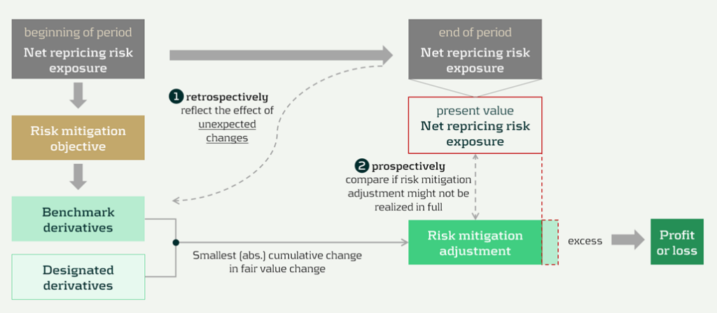
Figure 3 Risk mitigation adjustment and prospective and retrospective testing (source: IASB ED – Snapshot, December 2025)

The two tests are:

1. Benchmark adjustments for unexpected changes (retrospectively): First, benchmark derivatives must be adjusted when unexpected changes in the underlying portfolios reduce the net repricing risk exposure below the risk mitigation objective in a repricing time band (i.e., correction of overhedge), as they would otherwise no longer represent the repricing risk specified in the risk mitigation objective [7.4.6, B7.4.10].
2. Excess test to prevent unrealizable adjustments (prospectively): Second, an explicit excess assessment to prevent the risk mitigation adjustment from accumulating beyond what can be supported by the remaining net repricing risk exposure. If there is an indication that the accumulated risk mitigation adjustment may not be realized in full, the entity compares the risk mitigation adjustment to the present value of the net repricing risk exposure at the reporting date (discounted at the mitigated rate) [7.4.11–7.4.13]. This would happen if unexpected changes have not been fully reflected in the adjustments to the benchmark derivatives.

Any excess is recognized immediately in profit or loss by reducing the risk mitigation adjustment, and it cannot be reversed [7.4.14; BC101–BC103]. It acts like a safeguard: if revised behavioral assumptions shrink future repricing exposure, the unearned portion of the adjustment is released to P&L straight away.

Key considerations and insights

13. Operational burden (3/3) – benchmark derivatives: The reliance on ‘unexpected changes’ and time-band caps may force highly granular, frequently re-constructed benchmark derivatives, creating a mismatch versus designated derivatives. This could be operationally heavy, as noted by EFRAG.

14. Unclear testing and adjustment mechanics: The ‘excess’ framework is under-specified. Triggers and documentation expectations are unclear, and the present value test for net exposure is conceptually and operationally challenging, especially for modelled items (e.g., NMDs), as noted by EFRAG.

Discontinuation [ED 7.5]

Discontinuation is intentionally rare. RMA is not switched off because hedging activity changes. It only stops when the risk management strategy changes, and it stops prospectively from the date of change.

Key requirements include:

• Strategy: strategy triggers a change; activity does not. A change in how repricing risk is managed, such as changing the mitigated rate, changing the level at which repricing risk is managed (group vs entity), or changing the mitigated time horizon [7.5.1, 7.5.2].
• Prospective application: discontinue from the date the strategy change is made. No restatement of prior periods [7.5.1].

After discontinuation, the existing balance is recognized in profit or loss, either:

• Over time, on a systematic basis aligned to the repricing profile, if repricing differences are still expected to affect profit or loss [7.5.3(a)], or,
• Immediately if those repricing differences are no longer expected to affect profit or loss [7.5.3(b)].

Disclosures [IFRS 7]

The disclosures are meant to show, in a compact way, what risk is being mitigated, what derivatives are used, and what the model produced in the financial statements.

Key disclosures include:

• RMA balance sheet and P&L: risk mitigation adjustment closing balance and current-period P&L impact [30E].
• Risk strategy and exposure: repricing risk managed, portfolios in scope, mitigated rate and horizon, risk measure, and exposure profile [30H–30L].
• Designated derivatives: timing profile and key terms, notional amounts, carrying amounts, and line items, and FV change used in measuring the adjustment [30I, 30M].
• Sensitivity: effect of reasonably possible changes in the mitigated rate [30J].
  Volatility and roll-forward: FV changes not captured and where presented, plus reconciliation including excess amounts and discontinued balances [30N–30P].

Key considerations and insights

15- More, and more sensitive, disclosures: RMA adds extensive requirements (profiles, sensitivities, roll-forwards) that may reveal non-public positioning, so aggregation and materiality judgment matter.

Conclusions

The RMA proposal appears to be a constructive development toward reflecting the management of interest rate risk in dynamic portfolios more faithfully in financial reporting. Compared with existing approaches, it offers a clearer conceptual link between net repricing-risk management and accounting outcomes.

At the same time, several core mechanics might prove challenging in practice. In particular, further clarification would be helpful on the benchmark-derivative mechanism, the operation and trigger logic of the excess test, and the level of granularity and governance expected for the ongoing application. These areas will likely be central to implementation efforts, earnings volatility outcomes, and cross-bank comparability.
At this stage, practical outcomes may therefore differ significantly depending on interpretation and system design choices. Additional IASB guidance, informed by field testing and stakeholder feedback, could reduce that uncertainty and support more consistent application. Overall, RMA can be seen as a promising direction that improves conceptual alignment with risk management, while still requiring further clarification before its operational and reporting implications are fully settled.

The Proliferation of Valuation Models 

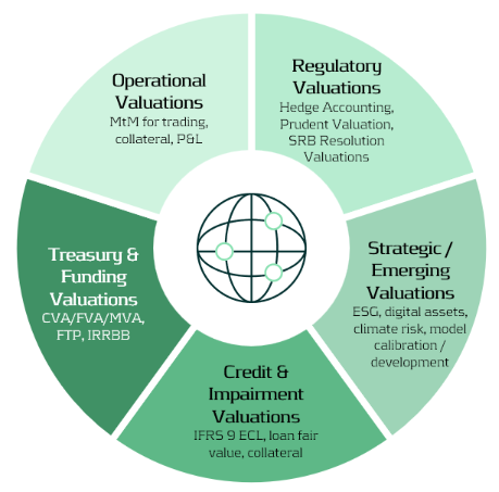
Valuation lies at the heart of financial institutions — informing decisions in trading, risk management, collateral management, accounting, and financial reporting. Yet across many banks, these valuations are performed in fragmented silos for different purposes, using different models, data sources, and systems. In addition to these core applications, valuations also support a broader range of activities, including treasury, regulatory reporting, and emerging domains such as ESG and digital assets.  

As illustrated in the Valuation Map (Figure 1), we observe that in many cases different departments conduct their own valuations, often for their own distinct purposes and using distinct valuation processes. Survey evidence shows that finance and FP&A teams devote roughly 65% of their time to data gathering, cleaning, and reconciliation, leaving only about 35% for value-adding analysis¹.

The Cost of Fragmentation 

Fragmented valuation architectures translate directly into higher costs and operational drag. In practice, three effects are most pronounced: 

• High data vendor spend –  market-data pricing surveys found that some firms were paying “many multiples” more than peers for similar products and use cases, reflecting redundant sourcing and poor usage visibility².

• Model proliferation – large banks often operate with hundreds to thousands of models across the enterprise, creating overlap in purpose and increasing governance, maintenance, and compute costs³. 

• Inconsistent and time-consuming valuations – disparate models and data feeds lead to unclear ownership of valuation “truth” and significant manual reconciliation between accounting, risk, and front-office views. 

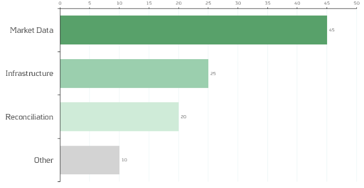
Although no public benchmark precisely mirrors our allocation, multiple industry surveys converge on the same conclusion: market data represents a dominant share of valuation costs, and fragmented reconciliation processes account for a significant portion of non-value-adding effort. Figure 2 therefore shows an indicative distribution — 45% market data, 25% infrastructure, 20% reconciliation, 10% other — to convey the relative scale of each component. Institutions will vary in mix, yet the implication is consistent: rationalizing data sourcing and automating reconciliation are among the highest-impact levers for reducing total valuation cost. 

Strategic Imperative: Centralizing and Standardizing Valuation 

Banks can unlock substantial efficiency gains by centralizing valuation logic and governing data flows. Similar to how treasury departments manage liquidity, banks should treat valuation processes as coordinated enterprise capabilities rather than fragmented operational activities.  

Key levers include: 

1-Valuation as a Service (VaaS): 

Establish a centralized valuation engine providing consistent pricing APIs for all functions (risk, finance, collateral, etc.). 

2-Unified Market Data Platform: 

Integrate vendor feeds into a single validated golden source with standardized identifiers and governance. 

3-Model Consolidation and Validation: 

Maintain one approved model per product type with clear ownership and lifecycle management. 

4- Process Automation: 

Automate reconciliation between accounting and risk views via shared data lineage and valuation transparency. 

5- Cost Transparency: 

Track valuation and data usage per business unit to encourage accountability and optimization. 

Together, these measures reduce duplication, accelerate reporting cycles, and improve consistency across valuation outcomes. 

Building the Foundation 

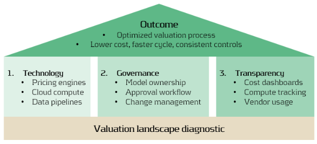
An optimized valuation operating model rests on three mutually reinforcing foundations:  

• Technology: Scalable pricing engines, cloud compute elasticity, and efficient data pipelines. 

• Governance: Clear model ownership, approval, and change management across risk and finance. 

• Transparency: Dashboards tracking valuation cost, compute time, and data provider usage. 

A practical first step: Zanders can perform a valuation landscape diagnostic, mapping all valuation types, systems, and data sources. Such analysis typically reveals 10–20% potential overlap and quick wins in data consolidation⁴. 

Conclusion: Elevating Valuation Processes to an Enterprise Capability 

In today’s environment of cost pressure and regulatory scrutiny, optimizing valuation processes is not only about efficiency—it is about strengthening consistency, transparency, and trust across the organization. Institutions that unify valuation workflows, data, and governance are better positioned to: 

• Reduce operational costs and reconciliation workloads. 

• Rationalize compute power – costs of running multiple models unnecessarily. 

• Strengthen governance and auditability. 

• Accelerate model deployment and reporting cycles. 

• Enable transparent, sustainable, and data-driven decision-making. 

At Zanders, we design and implement integrated valuation frameworks at leading financial institutions, that combine operational efficiency with regulatory robustness. 

If your organization is looking to streamline valuation processes, harmonize market data, or reduce reconciliation workloads, we invite you to connect with our experts.

Recent case law and regulatory developments provide useful guidance on what to expect in 2026 and on the approach that should be followed to mitigate the risk of challenges on intra-group loans.

Historically, tax authorities focused primarily on interest rate benchmarks when reviewing intra-group loans, cash pools and guarantees. Today, however, their analysis has become significantly broader and more sophisticated, extending to a range of interrelated factors such as contractual terms, debt capacity, and creditworthiness.

The sections below outline the key trends and risks shaping intra-group loan transfer pricing and highlight what multinational groups should address as part of their planning and compliance efforts for 2026.

Arm’s Length Terms & Conditions for Intra-Group Loans

Verifying that the terms and conditions of intra-group loans are consistent with how independent parties would contract remains a critical focus. In addition to establishing an arm’s length interest rate and the appropriate amount of debt (further explained below), it is also necessary to assess whether the other terms and conditions are at arm’s length. This involves considering the main features of the loan, and evaluating their impact on the risk profile of both the borrower and the lender, as well as on the arm’s length interest rate. Relevant terms that should be considered include currency, maturity, repayment schedule, and callability.

In 2025, courts emphasized that Transfer Pricing documentation must not only include a benchmark analysis but also a clear explanation of the contractual features agreed, especially for features such as subordination, maturity, interest structures, and repayment conditions. These features should align with the actual conduct of the parties and with the economic reality.

Multinationals have also seen a rise in challenges derived from discrepancies between the legal agreements drafted, the price applied between the entities involved, and the information presented in the Transfer Pricing report. A clear example is one-year loans that are automatically renewed, with the same price being applied and with no repayments being made, where tax authorities may reclassify them as longer-term arrangements, which typically carry a higher interest rate.

What to consider in 2026: It is important for multinational enterprises to carefully assess these terms and conditions before issuing a loan, as they will have a direct impact on the interest rate applied to the transaction. Drafting a comprehensive loan agreement that clearly outlines these terms, aligns with the conditions applied in practice, and is supported by a robust Transfer Pricing analysis is recommended to mitigate the risk of challenges by tax authorities.

Debt Capacity Analyses for Intra-Group Loans

Tax authorities are increasingly scrutinizing whether the amount of intra-group debt is economically justified and supported by a clear business purpose. They are also evaluating whether the debt aligns with arm’s length principles and serves a legitimate economic function consistent with the borrower’s overall business strategy.

A debt capacity analysis is often conducted to determine whether the borrower has the financial capacity to repay the loan and whether an unrelated party would provide a similar amount of financing under comparable conditions. If tax authorities consider that the amount of debt is excessive, adverse tax consequences could arise, such as the requalification of the debt as equity and/or the denial of a portion of the interest expense deduction.

Over the last two years, jurisdictions such as Germany and Australia introduced administrative guidelines formalizing debt capacity considerations. This trend has been further reinforced by case law in different countries over the past year. For example, in Luxembourg, a major hub for treasury companies and investment funds, the Luxembourg Administrative Court in 2025 issued a pivotal decision in case No. 50602C rejecting an automatic 85:15 debt-to-equity standard and holding that arm’s length analyses must be fact-specific and supported by data rather than mechanical ratios.

What to consider in 2026: Multinationals are expected to prepare robust debt capacity analyses for each borrower entity, demonstrating that independent lenders would extend a similar amount of debt. The debt quantum should be supported by financial projections, coverage ratios, and a documented business purpose, all included in the corresponding Transfer Pricing report.

Debt Capacity Analysis

A guide to demonstrating the arm’s length principle in debt financing

Get the whitepaper

Credit Rating Analyses for Financial Transactions: Stand-Alone vs Group Rating

Both tax administrations, and subsequently, courts, are scrutinizing the credit rating approaches applied by taxpayers in the context of intra-group loans. Credit rating analyses are a core step when pricing intra-group loans, as the risk profile of the borrower has a material impact on the applicable interest rate.

While simplified blanket ratings across a group were once tolerated, tax authorities and courts are now emphasizing the importance of entity-specific ratings adjusted for implicit support.

In Belgium, on June 6, 2025, the Court of First Instance of Leuven clarified that credit ratings must be substantiated and not merely assumed based on group affiliation. Based on this ruling, the borrower should be assessed on a stand-alone basis, taking into account the impact of the new debt quantum on its financial position. Where implicit group support is considered, it must be properly substantiated through a thorough implicit support analysis and cannot be assumed by default our automatically applied.

In the Netherlands, the Court of Appeal of Amsterdam, in its judgment of 11 September 2025, addressed, among other topics, the guarantee fees applied by the taxpayer and rejected their payment, emphasizing the importance of factoring implicit support into the credit rating applied to the borrower. This once again highlights the relevance of a two-step process: first, the calculation of the stand-alone rating, and second, the adjustment of this rating for implicit support.

As this is a highly relevant topic, and both the lender’s jurisdiction (seeking a lower credit rating, which drives higher interest income) and the borrower’s jurisdiction (seeking a higher credit rating, which drives lower interest expense) have opposing incentives, multinationals need to have a robust and consistent process in place.

What to consider in 2026: Companies should apply a consistent methodology for credit rating analyses based on the principles and best practices set out in Chapter X of the OECD Transfer Pricing Guidelines. Where possible, this involves performing an individual credit rating analysis for each borrower, adjusted for group implicit or explicit support. In addition, this analysis should be properly documented in the Transfer Pricing report.

Cash Pooling Structures and Synergy Allocation

Cash pooling structures remain an area of intense scrutiny by tax authorities worldwide. Cash pool Transfer Pricing analyses can be complex and time-consuming for a variety of reasons.

On the one hand, the participants’ accounts need to be priced on an arm’s length basis (considering the specific currency and the risk profile of each entity). This also includes identifying long-term structural balances and pricing them separately, where relevant. On the other hand, the cash pool leader needs to receive appropriate remuneration for the functions performed, risks assumed, and assets employed.

In addition, the OECD Transfer Pricing Guidelines state in paragraph 10.143 that: “The remuneration of the cash pool members will be calculated through the determination of the arm’s length interest rates applicable to the debit and credit positions within the pool. This determination will allocate the synergy benefits arising from the cash pool arrangement amongst the pool members and will generally be done once the remuneration of the cash pool leader has been calculated.”

Tax authorities are increasingly considering these recommendations, and this is becoming particularly relevant in jurisdictions where multinational enterprises have cash-rich pool entities, as tax authorities may expect that a portion of the synergies generated is allocated to them.

Finally, the involvement of multiple countries adds further complexity, as local jurisdiction-specific interpretations of the OECD Transfer Pricing Guidelines may arise. Over the past year, for example, a notable case was issued by the Spanish Supreme Court on July 15, 2025 (ruling 3721/2025). In its decision, the Court rejected the asymmetry of interest rates depending on whether they related to deposits made by the Spanish subsidiary or to amounts received by it as a loan, and emphasized that the remuneration of the leading entity must be consistent with its functions as a mere treasury centralization entity. This highlights the importance of following a coherent methodology based on the OECD Transfer Pricing Guidelines in order to support the position adopted in the event of a challenge by local tax authorities.

What to consider in 2026: Multinationals with cash pooling structures, especially where the amounts involved are material, should perform a Transfer Pricing analysis in line with the best practices set out in the OECD Transfer Pricing Guidelines. This includes: 1) pricing the debit and credit positions of the participants, identifying structural balances; 2) calculating the synergy benefits generated by the structure; and 3) allocating these synergies between the cash pool leader and the participants.

Key Takeaways for Intra-Group Loans Transfer Pricing in 2026

• Tax authorities are moving beyond interest rate benchmarking and increasingly focusing on the full arm’s length characterization of intra-group loans, including contractual terms and economic substance.
• Debt capacity analyses are becoming increasingly important, as evidenced by recent regulatory developments and case law.
• Credit rating analyses should be performed on a stand-alone basis and adjusted for implicit or explicit group support, in line with the OECD Transfer Pricing Guidelines.
• Cash pooling arrangements require careful allocation of synergies between participants and the cash pool leader based on functions, risks, and realistic alternatives.
• Robust and consistent transfer pricing documentation remains essential to mitigate the risk of challenges in an environment of heightened scrutiny.

Zanders Transfer Pricing Solution  

As tax authorities intensify their scrutiny of loans, cash pools, and guarantees, it is essential for companies to carefully adhere to the recommendations outlined above.Does this mean that additional time and resources are required? Not necessarily.

Technology provides an opportunity to minimize compliance risks while freeing up valuable time and resources. The Zanders Transfer Pricing Suite is an innovative, cloud-based solution designed to automate the Transfer Pricing compliance of financial transactions. 

With over eight years of experience and trusted by more than 100 multinational corporations, our platform is the market-leading solution for compliance with OECD Transfer Pricing Guidelines for intra-group loans, guarantees, and cash pooling arrangements.

You are currently viewing a placeholder content from YouTube. To access the actual content, click the button below. Please note that doing so will share data with third-party providers.

More Information

Unblock content Accept required service and unblock content

Our clients trust us because we provide: 

• Transparent and high-quality embedded intercompany credit rating models. 
• A pricing model based on an automated search for comparable transactions. 
• Automatically generated, 40-page OECD-compliant Transfer Pricing reports. 
• Debt capacity analyses to support the quantum of debt. 
• Cash Pool Solution which calculates the synergies generated by the structure.
• Legal documentation aligned with the Transfer Pricing analysis. 
• Benchmark rates, sovereign spreads, and bond data included in the subscription. 
• Expert support from our Transfer Pricing specialists. 
• Quick and easy onboarding—completed within a day!

As part of our ongoing series on the ECB’s 2026 Geopolitical Reverse Stress Test, we previously explored why channels matter more than numbers and how geopolitical risk shapes failure pathways in reverse stress testing.

Why This Matters

A key objective of the ECB’s 2026 Reverse Stress Test is for banks to assess the resilience of their business model. This requires a comprehensive taxonomy of geopolitical risk drivers linked to business impact via plausible transmission channels. Without this foundation, reverse stress testing becomes guesswork, blind to hidden vulnerabilities and hard to defend under supervisory scrutiny.

Step 1: Identify and Engage the Right Stakeholders

Creating a useful taxonomy is not a siloed exercise. It requires bringing together a cross-functional working group: risk management to define categories and metrics, treasury and finance to assess balance sheet sensitivities, business lines to validate exposures, geography and concentrations, compliance and legal to capture sanction regimes and regulatory constraints. Early engagement ensures the taxonomy reflects the bank’s unique business model and risk profile.

Step 2: Structure the Taxonomy Using a Layered Approach

The starting point is to move from broad geopolitical themes to tangible impacts. Begin by identifying high-level drivers such as sanctions, trade fragmentation, energy disruption or military escalation.

From there, think about how these drivers ripple through the organization—through financial markets, the real economy, and safety & security. The goal is to connect these channels to your business model and balance sheet exposures, and then drill down to measurable risk parameters like PD/LGD shocks or market sensitivities.

Step 3: Apply Robust Modeling Approaches and “Reverse-Orientation”

Once the taxonomy is defined, the next step is to make it actionable. Start with scenario-based analysis to explore plausible geopolitical shocks and their effects across channels. Then, use sensitivity screening to identify which sectors and counterparties are most exposed.

It is not uncommon for this exercise to yield a constellation of viable assumptions leading to the desired outcome; quantitative methods, such as Monte Carlo simulations or optimization methods, can aid in exploring the solution space and guide in the choice of the scenario which best fits the profile and narrative of your organization. The aim is not to build the most complex model but to ensure the taxonomy translates into meaningful insights for decision-making.

Step 4: Leverage External Data and Benchmarks

No taxonomy should be built in isolation. External data adds credibility and depth. Regulatory guidance from the ECB provides a clear baseline, while industry benchmarks and rating agency data can help calibrate sector sensitivities.

Geopolitical risk indices and historical stress events offer valuable context for scenario design. Combining internal insights with external references ensures your taxonomy reflects both supervisory expectations and real-world dynamics.

Step 5: Establish Governance and Documentation

Finally, governance is what turns a taxonomy into a trusted framework. This means securing board-level oversight, involving cross-functional committees, and maintaining clear documentation of assumptions and methodologies.

Regular updates are essential, as geopolitical risks evolve. A well-governed process not only satisfies regulatory scrutiny but also embeds the taxonomy into the bank’s risk culture, making it a living tool rather than a one-off exercise.

How Zanders Can Help

We guide banks through this process end-to-end:

• Quantitative modeling to support or benchmark scenario design.
• Advisory support to design and validate a complete taxonomy.
• Hands-on assistance during stress test exercises, leveraging experience with European banks.
• Tooling development or deployment of our Credit Risk Suite (CRS) for scenario modeling, automated ECL/CET1 impact calculations, and advanced optimization techniques.

Transform compliance into strategic capability for resilience. Contact us to find out how we can help your organization.

Read our previous blog on ECB 2026 Geopolitical Reverse Stress Test.

Why This Matters

For banks, the ECB’s 2026 thematic reverse stress test on geopolitical risk is more than a regulatory exercise. It’s a reality check on failure pathways. The cost of missing how shocks transmit through your business can be severe: capital depletion, liquidity strain, and reputational damage when the next crisis hits.

This is not about ticking boxes or plugging in generic macro scenarios. It is about demonstrating to supervisors and to your board that you understand which channels could break your business model and how those channels map to tangible impacts on capital, liquidity, and operations.

In reverse stress testing, you start from a pre-defined failure outcome and work backwards to plausible scenarios that could cause it. In our previous blog, we argued for a bank-specific taxonomy of geopolitical risk drivers because reverse stress testing is only credible when the transmission channels are correctly selected and explained. Today, we take the next step: translating a risk driver into business‑model impact that can credibly produce the failure condition.

Worked Example: Military Escalation

In the context of Military Escalation, as an illustrative example, let’s consider a conflict disrupting shipping lanes in the South China Sea. The chain of transmission may unfold as follows:

• The incident would disrupt global trade routes, creating severe supply chain¹ bottlenecks and driving up costs for  industries depending on imports from and exports to the region. These disruptions would ripple through the real economy, affecting manufacturing, logistics, energy and semiconductor² sectors, and ultimately impacting banks with concentrated exposures in these sectors.

• Investors would seek safe assets, triggering sharp movements in commodity and foreign exchange markets. Banks with open positions in these markets could face significant mark-to-market losses, while liquidity strains emerge as funding costs rise. In addition, cargo insurance premiums on conflict‑adjacent corridors can spike, prompting re-routing and a broader repricing of risk.

• Operational risks would likely increase. Military tensions often coincide with heightened cyber and/or physical threats, increasing the likelihood of state-sponsored attacks on financial infrastructure. Banks would need to increase investment in cyber defence and resilience measures.

• Sanctions may be imposed by multiple parties, exposing banks to potential breaches and contractual disputes with counterparties linked to conflict zones. This adds complexity to transaction screening and legal oversight.

• Finally, these channels translate into measurable risk parameters. Credit portfolios tied to vulnerable sectors would see severe PD shocks, alongside LGD adjustments for collateral impacted by trade restrictions. Together with the market and operational risk impacts described above, they could erode CET1 ratios, revealing failure pathways that standard stress tests might miss.

Reverse The Logic

Because a reverse stress test starts from the outcome, the final step is iterative - the engine room of the exercise. To reach the targeted impact (300 bps CET1 depletion in the ECB’s thematic exercise), you will likely cycle through the channel, mechanism, risk‑parameter mapping and tune the shocks, strengthening or weakening their severity and duration until the constellation of assumptions consistently delivers the failure condition. But a key fallacy is to treat this as a mechanic “tuning” exercise rather than a careful consideration of which combination of shocks and channels that plausibly will drive CET1 below the threshold?

Scaling This Approach

The method extends to other relevant drivers: sanctions, energy disruptions, cyber threats, but the taxonomy must be granular and defensible, with a clear line‑of‑sight from event to channel, and then to portfolio, risk parameters and capital metrics. This strengthens Reverse Stress Testing credibility and ICAAP alignment, and produces governance‑ready narratives for senior decision‑makers.

How We Can Help

We support banks in building a robust RST framework. Our approach includes:

• Advisory support to design a purposeful, bank-specific taxonomy and link it to ICAAP.
• Quantitative modeling to support or benchmark scenario design.
• Hands-on assistance during stress test exercises, leveraging our experience with several European banks.
• Tool development and deployment of our Credit Risk Suite (CRS) for scenario modeling, automated ECL and CET1 impact calculations, and advanced scenario building.

With Zanders, you can move beyond compliance to create a stress test framework that enhances your strategic capability.

On November 4, MeteoSwiss published updated climate scenarios for Switzerland. The scenarios describe the expected changes in the climate in Switzerland under an increase in global warming by 1.5, 2 and 3 degrees respectively (Global Warming Level (GWL)) compared to the reference period 1991-2020. The timing if and when these GWLs are reached depends on the specific climate scenario considered.  

The climate scenarios for Switzerland are anchored in the global climate scenarios that have been included in the sixth and last assessment report of the Intergovernmental Panel on Climate Change (IPCC) from 2022. The three main global scenarios considered are a combination of a Shared Socio-Economic Pathway (SSP) and a Representative Concentration Pathway (RCP): 

• “SSP1-2.6” represents a combination of SSP1 and RCP2.6 ("2-degree path with net-zero target achieved by 2050") 

• “SSP2-4.5” represents a combination of SSP2 and RCP4.5 (“’Middle ground’ scenario following current and planned measures“) 

• “SSP5-8.5” represents a combination of SSP5 and RCP8.5 (“Fossil fuel path without climate protection“) 

The Figure above depicts the approach taken by MeteoSwiss to assess the consequences for Switzerland at specific GWLs: 

1. The top part of the Figure (“Global”) shows three global climate scenarios, each of which achieves the depicted GWL at a different point in time. 
2. MeteoSwiss has translated each of the global scenarios to specific scenarios for Switzerland (more than three in fact, but the picture only shows three). These scenarios are shown in the bottom part of the Figure (“Swiss”). It can be seen that the same GWL in the global scenarios corresponds to different warming levels for Switzerland. This leads to a range of possible warming levels in Switzerland for each GWL. 

In the next sections, the main expected changes in temperature and precipitation in Switzerland under the different GWLs are considered. Subsequently, the steps needed to use the information about the climate scenarios for a materiality assessment of climate risk are outlined. In addition, an overview is provided of the data that has been made available for the Swiss climate scenarios by MeteoSwiss, which can be used for such a materiality assessment. 

1. Changes in temperature 

MeteoSwiss estimates that by 2024, the average temperature in Switzerland already increased by 2.9°C compared to pre-industrial times (1871-1900). This is more than double the rise of 1.4°C in average global temperature. The larger rise in Switzerland is partially due to the fact that the temperature above land increases more quickly than above sea. 

With rising global warming, the number of hot days (>30°C) in Switzerland is expected to roughly triple in a 3-degree world (GWL3.0). The largest impact will be in urban areas, as depicted in the Figure on the right.  

In line with this, the average summer temperature as well as extreme temperatures (warmest day and night) will increase. 

Potential economic consequences: 

• Extreme heat during the day and a lack of cooling at night put strain on the body and affect health. In addition, physical and mental work is made more difficult during heatwaves, with dense urban development exacerbating this. This will affect productivity, lower economic output and may increase costs for cooling work environments. 

2. Changes in precipitation 

Yearly precipitation is not expected to change in Switzerland with global warming, but summers are expected to get drier and winters are expected to get wetter. Moreover, extreme precipitation (heavy rainfall, hail) is expected to increase in both frequency and intensity, as depicted in the Figure below. 

Source: Climate CH2025 – Brochure, MeteoSwiss (link) 

Drier summers lead to an increased risk of forest fires as well as increasing frequency and intensity of droughts, as depicted in the Figures below. 

Precipitation in winter will increasingly fall in the form of rain instead of snow as the zero-degree line increases.  

Potential economic consequences: 

• Sudden flash floods and hail can cause property damage and business interruptions. In addition, they can destroy agricultural crops. This will negatively affect economic output and decrease the value of properties in areas at risk. 

• Drought leads to yield losses in agriculture and increased risk of forest fires, causes water shortages in reservoirs and restricts water supply. In addition, drought can intensify and prolong heatwaves. This will negatively affect economic output 

• Thawing permafrost and melting glaciers can lead to unstable slopes, and the water cycle may be disrupted. This will affect industries that depend on water (e.g., for cooling). Decreasing snow will also affect winter tourism and associated industry sectors. 

3. Estimating financial impacts 

For the potential future changes in temperature and precipitation in Switzerland because of global warming, the possible economic consequences have been explored in the sections above. To what extent these are relevant for risk management of a financial institution will depend on the sectors and physical locations of their clients, counterparties and issuers of securities in which they invest.  

The general steps taken to perform a materiality assessment for individual clients, counterparties and issuers are: 

1. Identify transmission channels through which the impacts of global warming can negatively impact their business. 

2. Estimate the financial impact of individual transmission channels. 

• As historical data is not representative of what is likely to happen in the future under global warming, a common approach is to use scenario analysis.  

• FINMA explicitly expects financial institutions to employ scenario analysis when performing the materiality assessment for nature-related financial risks in its recent circular (link, see our Zanders blog for a summary).  

• The Swiss climate scenarios can form a basis for the scenario analysis. However, the climate impacts that have been made available by MeteoSwiss (see Section 4) need to be translated to a financial impact for clients, counterparties and issuers. The impact on both revenues (e.g., lower sales due to business disruptions or lower demand) and costs (e.g., higher costs due to damages or required additional investments) need to considered. 

• Mitigating measures such as insurance can be taken into account if they are deemed effective in the scenarios considered. 

3. Reflect the estimated financial impact in internal risk metrics, such as credit ratings, collateral values and the value-at-risk of investments. 

For companies that are active internationally, or which depend on international supply chains, the exposure of their supply chains and international markets to the impact of global warming also needs to be considered. 

4. Swiss climate scenario data 

With the publication of the Swiss climate scenarios, MeteoSwiss also makes available detailed scenario data. This data can be viewed through an interactive WebAtlas (link) for combinations of: 

• Various temperature and precipitation indicators (listed in the document “Overview of CH2025 climate indicators” (link)) 

• Reference period (1991-2020) and three future Global Warming Levels (GWL1.5, GWL2.0 and GWL3.0) 

• Annual changes as well as seasonal changes (Winter, Spring, Sommer and Autumn) 

• Switzerland as a whole, each of five ‘biogeographic’ regions (Jura, Swiss Plateau, Pre-Alps, Alps, and South side of the Alps) as well as individual weather stations 

• Three climate scenarios (SSP1-2.6, SSP2-4.5 and SSP5-8.5) over time (2040-2060) (for mean temperature and precipitation only) 

The following detailed data can also be accessed directly: 

• Historical climate data (daily) at individual Swiss measurement stations since measurement started, covering 169 indicators related to temperature, humidity, precipitation, wind, sunshine, snow, air pressure, evaporation and radiation. (link) 
  • These data have been ‘homogenized’ for changes in measurement methods over time. 

• Scenario forecast data (daily) for different Global Warming Levels (GWL) under different Regional Climate Models (RMC) (link)(link) at 
  • Individual weather stations (DAILY_LOCAL) 
  • 1km×1km gridpoints in Switzerland (DAILY-GRIDDED) 

Climate variables included in the daily scenario forecasts are shown in the table below. 

How Zanders can help 

We have supported various banks with the assessment of the materiality of climate risks for their clients, counterparties and investment issuers. With our focus on risk and technology and our strength in applying quantitative approaches, we are particularly well equipped to substantiate a materiality assessment with scenario analysis and the use of data. If you want to learn more, do not hesitate to contact us. 

Introduction: Why This Matters Now 

Geopolitical risk has become a defining feature of today’s financial landscape. Trade fragmentation, sanctions, and regional conflicts are reshaping markets and business models. Recognizing this, the European Central Bank (ECB) will run a thematic Reverse Stress Test (RST) on geopolitical risk in 2026 as part of its explicit supervisory priorities. Unlike traditional stress tests, RST starts from a failure condition and works backward to identify plausible scenarios that could lead to this situation.  

Hence, this exercise is not about plugging in generic macro shocks—it’s about uncovering hidden vulnerabilities. And that requires one critical ingredient: an informed and detailed view of how geopolitical events may affect your organization. 

The Key Challenge: Seeing the Full Picture 

To pass muster with supervisors, selecting and explaining the transmission channels will matter far more than the numerical modeling. If relevant channels are missed, the backward search becomes blind, undermining the credibility of the entire exercise. The ECB has made clear that banks must go beyond traditional macroeconomic modeling and identify how disruption to trade flows and supply chains, cyberattacks, and even physical risks related to conflicts might affect banks and their clients, and in turn how this transmits to banks’ capital, liquidity, and operations.  

While the ECB has mapped out the primary pathways through which geopolitical risks propagate, the size and nature of the impact will very much depend on each bank’s location, exposures, and business models — meaning a one-size-fits-all approach will not work. Reverse stress testing is designed to uncover failure pathways, but this only happens if transmission channels have been studied and selected with care.  

Building a granular, bank-specific taxonomy of geopolitical risk drivers and their linkages to the portfolio is therefore a critical step. 

What Does a Geopolitical Risk Taxonomy Look Like? 

Well-defined transmission channels should link high-level risk drivers to specific impacts and risk parameters. For example: 

• Drivers: Trade tensions, sanctions, regional conflicts, cyber threats, energy disruptions, and overall market volatility. 

• Impacts: Credit losses (through direct and indirect exposures), loss of revenue (loss of markets, loss of pricing power), cost increases (funding costs, safety and security measures, insurance premiums, staff compensation and relocation), compliance and legal risks (sanctions breaches, disputes). 

• Risk Parameters: PD and LGD shocks, market risk factors, operational risk metrics. 

Once relevant transmission channels have been defined and quantified, the severity of the shocks to the risk drivers can be tuned so that the targeted reverse stress impact is achieved. In the case of the ECB reverse stress test, a CET1 capital impact of 300 basis points is targeted. Finding a balanced set of shocks to achieve the reverse stress target will require expert judgement and needs to be documented properly. 

A layered approach like this will help ensure that the exercise does not become a paper product but a strategic diagnostic tool that meets supervisors’ expectations. In our next blog, we will spend more time on how to set up a proper taxonomy and make it actionable for your organization. 

How Zanders Can Help 

At Zanders, we support banks in building a robust RST framework. Our approach includes: 

• Quantitative modeling to support or benchmark scenario design.  

• Advisory support to design a purposeful, bank-specific taxonomy and link it to ICAAP. 

• Hands-on assistance during stress test exercises, leveraging our experience with several European banks. 

• Tool development and deployment of our Credit Risk Suite (CRS) for scenario modeling, automated ECL and CET1 impact calculations, and advanced scenario building. 

With Zanders, you can move beyond compliance to create a stress test framework that enhances your strategic capability.

This article was first published on: TMI (Treasury Management International).

As the Swift MT-MX¹ co-existence phase came to a soft ending in November 2025, ISO 20022 (MX) messaging became the main standard for cross-border payment instructions between FIs. The migration will see the majority of cross-border payments moving from the legacy Swift FIN network to the Swift InterAct (FINplus²) network, with Swift providing an extension to the translation services where an FI has still not completed the migration to MX payment messages. Furthermore, last year, Swift started a pilot that would also allow the corporate community to access the FINplus network under a new Standardised Corporate Environment (SCORE) Plus model³. This article aims to demystify SCORE Plus as a possible additional or replacement Swift for corporates service and considers the key question – does it make sense for the corporate community to adopt?

Evolution of Swift for Corporates

The corporate community first gained access to Swift back in 1997 through the treasury counterparty model. This enabled corporates to receive the MT300 series messages covering FX confirmations. In 2001, corporate access evolved through the Member-Administered Closed User Group (MA-CUG) model. This enabled the corporate community to access the Swift FIN network covering the traditional MT-based messages in addition to the new Swift FileAct network, which supported file-based flows.

However, given the bank proprietary/bilateral nature of the MA-CUG model, this logically evolved into the SCORE model in 2006. SCORE offered the corporate community a more standardised and simplified implementation of the multi-banking model with access to both Swift FIN and FileAct networks.

Corporate adoption of Swift

From a corporate perspective, we have seen two primary adoption models:

• Swift FileAct only: under this corporate adoption model, vendor urgent and non-urgent payments, tax payments, treasury transactions, and in some cases payroll transactions are all sent to the cash management partner banks via FileAct. This standardised and secure file-based model simplified the corporate technology integration stack, with the flexibility to support both industry and bank proprietary payment, status reporting and balance and transaction reporting file formats. Importantly, performance wise, there was no material delay in the banking community processing urgent treasury payments under a file-based model, when compared with a separate Swift FIN network connection, with FileAct typically offering much richer file and transaction level status monitoring through the use of the ISO 20022 XML payment status report.
• Swift FIN and FileAct: this second corporate adoption model was typically linked to corporates that operated a TMS that only generated the Swift MT101 payment message. Individual treasury payments would be sent via the Swift FIN network, with vendor payments, tax payments, and possibly payroll transactions being generated within the ERP system and sent as a file using the Swift FileAct network. This adoption model required the corporate to subscribe to both the Swift FIN and FileAct networks.

Corporate adoption of XML messaging

An important point to underline at this stage is the corporate adoption of ISO 20022 XML messaging. A combination of the 2009 ISO standards maintenance release – commonly referred to as XML version 3, the underlying corporate motivation to simplify and standardise banking integration and finally the global industry collaboration – the common global implementation market practice group (CGI-MP⁴), which published a series of implementation guidelines.

These factors all contributed to XML payment messaging going mainstream in the corporate to banking domain. As the XML payment message (pain.001) could support almost any payment method globally, the corporate community embraced XML messaging for vendor payments, payroll, urgent payments, tax payments, and treasury transactions.

XML messaging enabled the corporate community to at least standardise the file format for making payments across the multi-banking environment, with the associated benefit of richer file and transaction status reporting.

Introduction of SCORE Plus

SCORE Plus, which came on-stream last year, is being labelled as an enhanced Swift for corporates adoption model, which provides more detailed and structured data for payments and reporting, combined with real-time transaction tracking and management, offering corporates improved visibility into their payment life cycle.

However, this reference to improved data is directly linked to the corporate migration onto ISO 20022 XML standard from the legacy MT101 FIN message. As noted above, the corporate community adoption of ISO 20022 XML messaging is already mainstream – globally. Second, taking the current cross-border payment services into account, payment tracking is already available today through the Swift Gpi service⁵ which enables the tracking through to the beneficiary bank account being credited.

The table below (fig. 1) seeks to highlight some of the key differences between SCORE (FileAct) and the enhanced SCORE Plus solutions from a corporate community perspective.

What is the impact to the corporate community?

While the below table provides a simple overview of the key differences, it’s important to understand what this means in practice to the corporate community, as there are some significant considerations:

• XML Version 9 payment message: first and foremost, any corporate looking to adopt SCORE Plus will have to develop the new XML version 9 payment message (pain.001.001.09), which was introduced as part of the ISO 2019 annual standards maintenance release. While this SCORE Plus development will permit other domestic payment methods, which can be defined through use of the service level code, users are limited to sending just one transaction per file. This single transaction limitation follows the same logic as the legacy FIN MT101 payment message, despite the richness and flexibility of the underlying XML V09 payment message, which has almost 1,000 XML data tags.
• Business Application Header: in addition to developing the new XML V09 payment message, there is an additional Swift requirement to also include the Business Application Header (BAH), which contains sender and receiver information. The BAH is not required where the XML V09 payment message is sent under the traditional FileAct connection.
• Swift network validation: strict network messaging validation will apply to all SCORE Plus messages. While this might sound like a benefit, migrating to the new XML V09 message will logically and ultimately embrace the other payment methods that can be sent in bulk – so domestic non-urgent, instant, domestic urgent, tax, and potentially payroll transactions that will be sent via Swift FileAct. A key guiding principle of the CGI-MP group was data over-population, which both simplified the design and development of XML payment messaging, and also enabled a core multi-banking XML template to be agreed with core banking partners. This approach is particularly beneficial where a corporate maintains a global master vendor record, which typically contains both domestic clearing and international bank routing codes in addition to full address information. This approach allows more information to be provided in the XML payment message as part of an agreed template, with the originating banking partner accepting and ignoring any surplus data that is not relevant for the requested payment method. Although there does appear to be some flexibility under the SCORE Plus model, this is an area that needs to be carefully considered as part of any adoption decision in order to ensure messages that contain data over-population will not be rejected by the Swift network. This means the corporate community will need to closely review the published Cross-Border Payments and Reporting Plus (CBPR+) industry guidelines⁶ to determine any possible friction points.
• Remittance Information: SCORE Plus will support up to 9,000 characters of payment remittance information, however this can only be provided in either the structured or unstructured xml tags. Users are not permitted to use both structured and unstructured within the same payment message. This is in contrast to the Swift FileAct model, which will allow the corporate community to populate both structured and unstructured xml tags within the same payment instruction.
• Message Design: when the XML payment message was designed, it provided flexibility for the corporate community to decide whether to specify elements such as the payment method, ultimate debtor, and charge bearer code at batch or individual transaction level. This flexibility allowed for a more efficient payment message design as a file containing 10,000 non-urgent payments could be defined once using the service level code NURG at the batch level as opposed to 10,000 times at a transaction level. Now while SCORE Plus is crystal clear that only single transactions can be sent within each file, which removes any issue, this does mean the corporate community will need to design a completely different XML V09 message for the Swift FileAct flows adding additional complexity and cost.
• Status Monitoring: in terms of the status monitoring and tracking capabilities, SCORE Plus provides options, which translate into additional development. The first option is to use the new XML V10 payment status report, which, subject to partner bank capabilities, will incorporate the Swift Gpi end-to-end tracking for cross-border payments. Alternatively, or in addition to the payment status report, Swift will be introducing the new TRCK.004 payment tracking message, which will provide improved end-to-end visibility around cross-border payments. The new tracking message will be released as part of the November 2026 standards release (SR2026). Although this initially sounds positive, it’s important to remember that the Swift Gpi service enables tracking through the intermediate banking partners through to the beneficiary bank account being credited. Furthermore, the new XML V10 payment status report will still be required for the Swift FileAct flows whenever the corporate decision is taken to migrate to the XML V09 payment message. Ultimately, this could mean two types of status and tracking messages will have to be developed, contributing to the overall cost and time taken to complete any development.

Key questions corporates should be asking themselves

The first question is what is the reason behind considering SCORE Plus? If a business is currently sending the MT101 message via Swift FIN, there is currently no industry-agreed end date to the corporate community sending the MT101 payment message to partner banks. However, given the November 2026 end date for providing the unstructured postal address, this might require some fine tuning in the form of adopting Tag 59 option F. This Swift-agreed industry workaround permits the corporate community to send structured postal address data, subject to specific formatting rules. The Tag59F approach provides a light-touch way of achieving compliance as the actual development is limited to a field-level change in addition to some master data address clean-up work. And full compliance means providing the minimum mandatory postal address data requirements⁷ – city/town name and ISO country code.

Alternatively, the reason might be to replace the existing Swift FIN network connection with the new SCORE Plus network. If this is the case, it is important to consider whether there is an existing Swift FileAct connection to send payment messages. The benefit of potentially extending the use of the existing FileAct connection to also make cross border payments is twofold.

1. It removes the immediate requirement to develop the new XML V09 payment message, BAH and associated new tracking messages.
2. It now allows the consolidation of Swift services to just a Swift FileAct service and thereby reducing overall Swift membership costs.

Conclusion

SCORE Plus has been designed as a replacement for the legacy Swift FIN network. While the benefits are mainly associated with a corporate migration from the MT101 message to the new XML V09 payment message, this does not recognise that XML messaging is already mainstream within the corporate community – with Swift FileAct typically supporting a multi-banked file-based interface.

There are also alternative approaches to address the forthcoming November 2026 compliance deadline – both a light touch for MT101 users, while existing XML V03 (version 3) message users can add cross-border payments as a new payment method and configure either the hybrid address or full structured address and continue to send via Swift FileAct or bank proprietary host-to-host connection.

An additional material risk is the pending decision on whether corporates that adopt SCORE Plus will also have a mandatory requirement to keep aligned to the latest version of the XML payment message. Discussions are planned for December 2025, but if the decision is taken to force corporate users to align to the annual ISO standards maintenance release, this will create a significant cost overhead on corporate users, with questionable benefits.

It’s also important to note that the associated XML V08 bank statement (camt.053.001.08) is currently in pilot-only mode and is subject to release later this month. As the SCORE Plus network has a bandwidth limit of just 100Kb, this translates to approximately 250 transactions that can be reported per bank statement message. This limitation does not exist under the FileAct network.

So, recognising the typical cost pressures within the corporate domain, further internal questions must be asked before formalising a plan to adopt SCORE Plus. It’s important that an informed decision is made around this key architectural change, as it impacts the connectivity, messaging, and associated payments workflow.

Does the commercial business case really stack up, or is now the time to think about if and when rationalising the current Swift for corporates services makes sense?

References

BCBS. (2004). International Convergence of Capital Measurement and Capital Standards. Bank for International Settlements.
Biche, E. (2022). A Probabilistic Approach to Quantify Margin of Conservatism for Data Deficiencies in a Calibration Sample for Credit Scoring Models.
EBA. (2017). Guidelines on PD estimation, LGD estimation and the treatment of defaulted exposures. European Banking Authority.
Hampel, F. (1974). The influence curve and its role in robust estimation.
Risk Trends 2026 Whitepaper
Read Zanders leadership's strategic outlook on risk's most crucial trends.
Download
Cash is back at the top of the agenda.
In a more volatile, fast-moving environment, treasurers are expected to make faster, better-informed liquidity decisions. Yet many organizations still rely on end-of-day visibility, fragmented systems and manual processes. This gap creates both risk and opportunity. Real-time liquidity is emerging as a practical way to strengthen control, reduce inefficiencies and support better financial decision-making.
Why treasurers are rethinking liquidity
For many years, treasury operated in a relatively stable environment. Payment cycles were predictable, processes were structured, and end-of-day visibility was sufficient to support most liquidity decisions.
Today, that model is under pressure. Funding conditions can tighten quickly, business needs can shift suddenly, and critical payment flows often require faster response times. At the same time, liquidity is no longer confined to traditional business hours. In a 24/7 economy, money can move at any moment, creating both new opportunities and additional complexity. This shift is not only driven by uncertainty. It also reflects a broader transformation in how businesses operate. Speed, immediacy and availability have become the norm, and expectations of treasury have evolved accordingly.
As a result, treasury is taking on a broader role. Beyond managing payments and reporting balances, treasurers are increasingly expected to support funding decisions, capital allocation and overall business resilience. This growing responsibility requires more timely, accurate and actionable information. This evolution is also reflected in recent industry research, highlighting the increasing strategic importance of treasury within the CFO organization with 63% of survey respondents indicating that the priority of Treasury function within CFO Office has increased over the past 5-10 years.
However, many treasury functions still rely on limited visibility, fragmented banking and ERP landscapes, manual processes and static, backward-looking forecasts. To compensate for this, organizations often maintain significant precautionary cash buffers. While these buffers reduce risk and ensure operational continuity, they also trap liquidity and increase inefficiencies. In practice, capital is not always deployed where it creates most value.
Why is liquidity management changing?
The environment is becoming more supportive of a more dynamic approach to liquidity management. Instant payments are a clear example. As they become increasingly standard across the euro area, liquidity can move more quickly and more flexibly, with less reliance on cut-off times.
At the same time, improvements in connectivity are reshaping treasury operations. APIs, host-to-host solutions and integrated banking platforms make it easier to access timely and reliable data. Intraday reporting provides better visibility throughout the day, rather than only at the end of the day. Treasury systems have also evolved, with stronger forecasting and automation capabilities. While none of these developments alone fundamentally transforms treasury, together they create the opportunity to manage liquidity in a more pro-active and flexible way.
What real-time liquidity actually means
Real-time liquidity is not about making every treasury activity instantaneous. Its value lies in increased certainty and control when it matters most. In practice, this means having better visibility on cash positions during the day, knowing whether payments have been made, and being able to act without delay when needed. This allows treasury teams to move from reacting after events to actively steering outcomes.
The value becomes particularly clear in high-impact situations. Payroll, critical supplier payments, debt servicing or M&A-related transactions all require a high degree of confidence that liquidity is available at the right place and at the right moment. In these situations, delays or manual interventions are not just inefficient. They can create real risk.
At the same time, real-time liquidity is not purely a technology question. Data availability, internal processes, governance and system integration all play a key role in determining whether the potential benefits can be realized.
A pragmatic path forward: How can organizations implement real-time liquidity?
For most organizations, real-time liquidity is best approached as a gradual evolution rather than a one-off transformation. A first step is to identify where faster and more accurate liquidity insights would create the most value. This helps prioritize efforts and ensures a clear link with business needs. The next step is to strengthen the foundations. Improving visibility across accounts, ensuring timely access to payment status information and simplifying account structures are essential building blocks.
Equally important is the treasury operating model. Faster infrastructure only delivers value if decision-making processes and governance are aligned. Clear roles, responsibilities and escalation paths make it possible to translate improved visibility into effective action.
Finally, forecasting remains a key complementary capability. A forward-looking view allows treasury to anticipate liquidity needs, reduce reliance on buffers and make better use of available cash.
Rather than aiming for a large-scale transformation from the onset, many organizations benefit from focusing on a limited number of high-impact use cases. This makes it possible to demonstrate value quickly and build momentum over time.
What's next
Real-time liquidity is a maturity journey rather than a destination, guided by business objectives and organizational complexity. It starts with better visibility and builds through greater confidence, stronger processes and improved control.
Value is created when better visibility builds confidence - confidence enables timely action and better decisions. Organizations that move early and pragmatically will not only manage volatility more effectively but also position treasury as a stronger strategic partner to the business.
Cash may be king again, but the real prize lies in what organizations can do with it when they are able to act in time.
This article was developed jointly by ING and Zanders, combining a banking perspective on real-time liquidity infrastructure with practical treasury transformation expertise.
ING Wholesale Banking serves large corporate clients, financial institutions, and governments across the globe, providing tailored solutions in areas such as lending, transaction services, and financial markets. With deep sector and sustainable finance expertise and people on the ground in many markets, ING Wholesale Banking supports its clients in navigating complex financial challenges and achieving their strategic objectives.
Zanders is a global advisory specialized in treasury management, financial risk management and treasury technology. It advises corporates, financial institutions and public sector organizations on treasury strategy, operating models, technology selection and implementation, and risk management.
Curious how real-time liquidity could apply to your organization?
Contact us
CEO and Managing Partner Laurens Tijdhof describes the origins and importance of Zanders’ purpose.
In 1994, Zanders was born in complexity.
From our very first clients, we worked in environments defined by large, capital-intensive balance sheets, fundamental transformation, and a growing need for professional treasury and risk management. These were never simple situations, and they never pretended to be.
That early exposure shaped our DNA.
Our clients operated where the stakes were high, decisions had real consequences, and financial performance truly mattered. They didn't need generic advice or temporary capacity. They needed a trusted advisor, someone who could make sense of complexity and help them act with confidence. That is where Zanders learned to be who we are today.
More than thirty years on, the world has changed, but the nature of the challenge has not.
Volatility is no longer cyclical, it is structural. Geopolitical tension, financial market disruption, regulatory pressure, and rapid technological change now converge. And they show up directly in the decisions CFOs, CROs, and leaders across treasury and risk have to make.
In that environment, the key question is no longer "What is happening?"
It is "What should we do about it, now?"
Our purpose speaks directly to that moment.
We help clients solve complex problems. We add value by delivering financial performance. Not when it is easy, but when it counts. And we help leaders strengthen liquidity, manage risk, and optimize capital to make better decisions today and stay in control tomorrow.
Complexity is also where opportunity lives. Digitalization, tokenization, and artificial intelligence are reshaping treasury and risk functions. When approached strategically, they unlock real advantage - in efficiency, resilience, performance, and decision speed.
At Zanders, we help clients reduce exposure where it matters most and unlock value where it truly exists. Always anchored in real-world challenges. Always focused on outcomes.
Laurens Tijdhof
CEO & Managing Partner, Zanders
Digital transformation is reshaping corporate treasury, but it is also exposing organizations to a faster, more sophisticated fraud and cybercrime threat landscape.