
This paper explores vital infrastructure decisions, regulatory scrutiny, and proposes a flexible risk approach for financial institutions in crypto asset navigation by 2025.
This paper offers a straightforward analysis of the Basel Committee on Banking Supervision's standards on crypto asset exposures and their adoption by 2025. It critically assesses infrastructure risks, categorizes crypto assets for regulatory purposes, and proposes a flexible approach to managing these risks based on the blockchain network's stability. Through expert interviews, key risk drivers are identified, leading to a framework for quantifying infrastructure risks. This concise overview provides essential insights for financial institutions navigating the complex regulatory and technological landscape of crypto assets.

This article explores the growing interest in sustainability among consumers and investors, the role of financial institutions in supporting green initiatives, and the rising concern about “greenwashing” – deceptive claims regarding environmental efforts by some financial institutions.
In recent years, consumers’ and investors’ interest in sustainability has been growing. Since 2015, assets under management in ESG funds have nearly tripled, the outstanding value of green bonds issued by residents of the euro area has surged eightfold, and emission-related derivatives have seen a more than sevenfold increase1.
The global push for sustainable and environmentally responsible practices has led to an increased focus on the role of financial institutions in supporting green initiatives. One of the ways financial institutions use to incentivise sustainable investments, is by designing new products, such as blue bonds to protect marine areas and other sustainability-linked bonds2, or by transitioning to funding sectors with positive sustainability impact.
However, amidst the growing wave of environmental consciousness, the credibility of "green" claims made by some financial institutions is a point of concern. This phenomenon, known as greenwashing, is gaining attention, not only within financial institutions, but also with regulators. Financial regulators, including the European Supervisory Authorities (ESAs) and UK’s Financial Conduct Authority (FCA) have taken action against potentially misleading green statements made by institutions. Despite these regulatory interventions, the persistent risk of greenwashing persists, primarily due to the absence of consistent standards governing sustainability claims and disclosures. The lack of uniform criteria poses an ongoing challenge to effectively combatting greenwashing practices within the financial landscape.
Defining Greenwashing
The ESAs describe greenwashing as “a practice where sustainability-related statements, declarations, actions, or communications do not clearly and fairly reflect the underlying sustainability profile of an entity, a financial product, or financial services. This practice may be misleading to consumers, investors, or other market participants” 3.
Financial institutions, as key players in the global economy, play a crucial role in fostering sustainability. However, some have been accused of using deceptive practices to push their green image without making substantial changes. This practice may be misleading to consumers, investors, and other market participants.
In practice, greenwashing can take different forms depending on the institution. For insurance companies, the European Insurance and Occupational Pensions Authority (EIOPA) found in their Advise to the European Commission on Greenwashing4 various examples where insurers misleadingly claimed to be transitioning their underwriting activities to net zero by 2050 without any credible plans to do so. Other examples include insurance companies falsely claiming to plant trees for each life insurance policy sold but failing to fulfil this promise, or products being marketed as sustainable merely because of a positive "ESG rating," despite the rating not taking into account any actual sustainability factors and focusing solely on financial risks.
Withing the banking sector, the EBA reported5 that the most common misleading claims relate to the current approach to integrating sustainability into the business strategy, claims on the sustainability results and the real-world impact, and claims on future commitments on medium and long-term plans.
Finally, for investment companies and pension funds, the European Securities and Markets Authority (ESMA) reported6 that most the common greenwashing practices result from exaggerated claims without any proven link between and ESG metric and the real-world impact.
Key Indicators of Greenwashing:
- Vague and Ambiguous Language: Financial institutions engaging in greenwashing often use vague terms and ambiguous language in their marketing materials. This lack of clarity makes it challenging for consumers to discern the actual environmental impact of their investments.
- Lack of Transparency: Genuine commitment to sustainability involves transparency about investment choices and the environmental impact of financial products. Institutions that are less forthcoming about their practices may be concealing less-than-green investments.
- Inconsistent Policies: Greenwashing is also evident when there is a misalignment between a financial institution's sustainability claims and its actual policies and practices. Actions, or lack thereof, can speak louder than words.
The Role of Regulatory Bodies
Greenwashing poses potential reputational and financial risks for the institutions involved. Addressing greenwashing might not only improve consumer’s trust in the products and services offered by financial institutions, but also will allow customers to make informed decisions that are align with their sustainability preferences and increase the capital into products that genuinely represent a more sustainable choice and drive a positive change. Tackling greenwashing should therefore be a priority for regulatory supervisors.
The introduction of the EU’s Taxonomy Regulation and the Sustainable Finance Disclosure Regulation (SFDR) addresses the initial concerns of greenwashing within the financial sector. The Taxonomy determines which economic activities are environmentally sustainable and addresses greenwashing by enabling market participants to identify and invest in sustainable assets with more confidence. SFDR promotes openness and transparency in sustainable finance transactions and requires Financial Market Participants to share the environmental and social impact of their transactions with stakeholders. In May 2023, the ESA published their progress report on greenwashing monitoring and supervision7. The report aims to provide insights into an understanding of greenwashing and identify the specific forms it can take within banking. It also evaluates greenwashing risk within the EU banking sector and determines the extend to which it might be and issue from a regulatory perspective.
In the UK, the FCA published in November 2023 a guidance consultation on the Anti-Greenwashing Rule8. The anti-greenwashing rule is one part of a package of measures introduced through the Sustainability Disclosure Requirements (SDR). The anti-greenwashing rule requires FCA-authorised firms to ensure that any claims they make to the sustainability characteristics of their financial products and services are consistent with the actual sustainability characteristics of the product or service and are fair, clear and not misleading, and have evidence to back them up. The propose rule will come into force on 31 May 2024.
While the existing and planned regulation contributes to addressing aspects of greenwashing, several measures have not yet fully entered into application, making the impact of the frameworks not visible yet. Beyond disclosures, regulators should also focus on tightening requirements on sustainability data and ratings, and creating mandates to prevent misleading statements and unfair commercial practices.
Going forward, as regulators gain more experience to comprehensively address greenwashing, financial institutions should expect increased supervision and enforcement of sustainable finance policies aimed at preventing misleading sustainability claims.
Actions to mitigate greenwashing risk
One of the biggest challenges financial institutions faced in relation to sustainability is that scientific progress, policy development and social values are in constant evolution. What was a well-supported green initiative two years ago can potentially be considered as greenwashing today.
In the meantime that stricter regulations and guidance is in place, financial institutions should take a broad view on how to develop and communicate sustainability strategies to mitigate greenwashing risk.
Here are three ways on how to prevent greenwashing:
- Promote disclosure: financial institutions should publish comprehensive sustainability reports and disclose ESG information as part of their financial reports.
- Commit to transparency: claims about environmental aspects or performance of their products should be justified with science-based and verifiable methods. Financial institutions should be transparent about their ambitions, status, and be open about any shortcomings they identified.
- Align business practices with purpose: financial institutions should determine which climate-related and environmental risks impact business strategy in the short, medium and long term. They should reflect climate-related and environmental risks in business strategies and its implementation. In addition, they should balance sustainability ambitions with the reality of real transformation.
Zanders’ approach to managing reputational risk
Avoiding greenwashing should always be a priority for institutions. If a risk arises in this area, reputational risk management can help to limit negative effects. Due to the interdependencies between ESG, reputational, business and liquidity risk, the supervisory authorities are also increasingly focusing on this area.
In the context of reputational risk management, we recommend a holistic approach that includes both existing and new business in the analysis. In addition to identifying critical transactions from a reputational perspective, the focus is also on active stakeholder management. This requires cross-departmental cooperation between various units within the institution. In many cases, the establishment of a reputation risk management committee is key to manage that topic properly within the institution.
Conclusion
While many financial institutions genuinely strive for sustainability, the rise of greenwashing highlights the need for increased vigilance and scrutiny. Consumers, regulators, and industry stakeholders must work together to ensure that financial institutions align their actions with their environmental claims, fostering a truly sustainable and responsible financial sector.
Curious to learn more? Please contact: Elena Paniagua-Avila or Martin Ruf
Citations
- European Central Bank, Climate-related risks to fiancial stability, 2021. ↩︎
- European Central Bank, Climate-related risks to fiancial stability, 2021. ↩︎
- European Banking Authority, Progress report on greenwashing monitoring and supervision, 2023. ↩︎
- European Banking Authority, Progress report on greenwashing monitoring and supervision, 2023. ↩︎
- European Banking Authority, Progress report on greenwashing monitoring and supervision, 2023. ↩︎
- European Securities and Markets Authority, Progress report on greenwashing, 2023. ↩︎
- European Banking Authority, Progress report on greenwashing monitoring and supervision, 2023. ↩︎
- Financial Conduct Authority, Guidance on the Anti-Greenwashing rule, 2023. ↩︎

Model risk from risk models has become a focal point of discussion between regulators and the banking industry.
Model risk from risk models has become a focal point of discussion between regulators and the banking industry. As financial institutions strive to enhance their model risk management practices, the need for robust model risk quantification becomes paramount.
An introduction to model risk quantification
Many firms already have comprehensive model risk management frameworks that tier models using an ordinal rating (such as high/medium/low risk). However, this provides limited information on potential losses due to model risk or the capital cost of already identified model risks. Model risk quantification uses quantitative techniques to bridge this gap and calculate the potential impact of model risk on a business.
The goal of a model risk quantification framework
As with many other sources of risk within a financial institute, the aim is to manage risk by holding capital against potential losses from the use of individual models across the firm. This can be achieved by including model risk as a component of Pillar 2 within the Internal Capital Adequacy Assessment Process (ICAAP).
Key components of a quantification framework
An effective model risk quantification framework should be:
- Risk-based: By utilising model tiering results to identify models with risk worth the cost of quantifying.
- Process driven: By providing a system for identifying, measuring and classifying the impact of model risks.
- Aggregable: By producing results that can be aggregated and including a methodology for aggregating model results to a firm level.
- Transparent & capitalised: By regularly reporting aggregated firm-wide model risk and managing it using capitalisation.
Blockers impeding model risk quantification
Complications of quantification include:
- Implementation and running costs: Setting up and regularly running any quantification test involves significant resource costs.
- Uncovered risk: Trying to quantify all potential model risk is a Sisyphean task.
- Internal resistance: Quantification and capitalisation of model risks will require increased resources to produce, leading to higher costs, making it a hard initiative to motivate individuals to follow.
Concepts in Model Risk Quantification
Impacts of Model Risk
Model risk significantly influences financial institutions through valuations, capital requirements, and overall risk management strategies. The uncertainties tied to model outcomes can have profound impacts on regulatory compliance, economic capital, and the firm's standing in the financial ecosystem.
Model tiering
Model tiering is a qualitative exercise that assesses the holistic risk of a model by considering various factors (e.g. materiality, importance, complexity, transparency, operational intricacies, and controls).
The tiering output grades the risk of a model on an ordinal scale, comparing it to other models within the institute. However, it doesn't provide a quantitative metric that can be aggregated with other models.
Overlap with quantitative regulations
Most firms already perform quantitative processes to measure the performance of Pillar 1 models that impact the regulatory capital held (such as the VaR backtesting multiplier applied to market risk RWA).
Model Risk Quantification Framework - The Model Uncertainty Approach
A crucial step in building a robust model risk quantification framework is classifying and assessing the impact of model risk. The model uncertainty approach is an internal quantitative approach in which model risks are identified and quantified on an individual level. Individual model risks are subsequently aggregated and translated into a monetary impact on the bank.
Regulatory Model Risk Quantificaiton Methods - RNIV, Backtesting Multiplier, Prudent Valuation and MoC
Most banks are already familiar with quantification techniques recommend by regulators for risk management. Below we highlight some of these techniques that can be used as the basis for expansion of quantification within a firm.
Expanding Model Risk Quantification
Our approach to efficient measurement relies on two key components. The first is model risk classifications to prioritize models to quantify, and the second is a knowledge base of already implemented regulatory and internally developed techniques to quantify that risk. This approach provides good risk coverage whilst also being extremely resource efficient.
Looking to learn more about Model Risk Management? Reach out to our experts Dr. Andreas Peter, Alexander Mottram, Hisham Mirza.

This article describes the current status of the IFRS 9 landscape, six years after the IFRS 9 accounting standards replaced IAS 39.
We touch upon the main difficulties experienced by financial institutions in the Netherlands based on a combination of project experience, results of a survey, main attention points from the eyes of the regulator and observations from publicly available annual reports. Interested to learn more about the IFRS 9 framework components banks struggle with the most and whether these challenges can be easily solved? Find out in the remainder of this article.
Introduction
The main objective of this article is to provide insight into market practices and common challenges within the IFRS 9 landscape of Dutch financial institutions. In this light, Zanders conducted a survey amongst Dutch financial institutions. Six main IFRS 9 framework components form the basis of the survey: data quality, model components (PD, LGD, EAD), SICR & staging, macroeconomic scenarios, out-of-model adjustments and the relation between IFRS 9 and other models within the bank. An example of a full IFRS 9 framework overview is presented in Figure 1. The questionnaire was followed up by a roundtable in which the most noticeable results from the survey were discussed with the participants.
Besides the survey, the IFRS 9 monitoring report published by the European Banking Authority (IFRS 9 Monitoring report, EBA (November 2023)) provides insights into the key IFRS 9 attention points from a regulatory perspective (e.g. as identified by EBA). In this article, we discuss the key differences between the difficulties experienced by banks versus attention points highlighted in the monitoring report. Lastly, this article uses publicly available information from annual reports to illustrate the diverging modeling practices and model behavior amongst market peers.
Figure 1: IFRS 9 framework overview.
Survey
The IFRS 9 survey held in Q4 2023 was centered around the six framework components as stated in the introduction section and which are graphically presented in Figure 1. The participating banks were asked in which areas of the framework they experience difficulties. Consequently, each area was explored deeper by means of questions directly related to each area.
All participating banks except one indicate difficulties in the areas of data quality and out-of-model adjustments (e.g. overlays). For data quality, changing policies (e.g. Definition of Default, loan quality assessment), limited loss realizations for LGD (as well as limited detail of the loss realization data) and dealing with unrepresentative data from the Covid-19 period are examples of reasons for the difficulties experienced in this area. With regards to out-of-model adjustments, it becomes apparent that many banks struggle with pressure from the regulator and audit, triggering banks to find an escape in overlays on the IFRS 9 model outcomes. Overlays are applied on a wide variety of topics, in various ways (e.g. calculated, constant, periodic, expert based, etc.) and sometimes constitute the majority of the total provisions. Altogether, this illustrates the need to have out-of-model adjustments in place that are sufficiently qualitatively substantiated and, whenever possible, are applied on the model component level. At the same time, we are of the opinion that out-of-model adjustments are sometimes over-used to make up for model deficiencies. Especially when out-of-model adjustments constitute the majority of the total provisions, compliance of the model with the IFRS 9 best-estimate principle should be questioned.
Surprisingly, only one third of the respondents experiences difficulties in the framework areas that came into existence with the introduction of IFRS 9; SICR & staging and macroeconomic scenarios. A possible explanation for this is that the responsibility for these framework areas is often distributed across multiple departments. Macroeconomic predictions and scenario weights are usually determined by a separate macroeconomic scenario department or committee, and staging assessments are often placed outside the scope of IFRS 9 modeling teams. From a governance perspective, we are of the opinion that more alignment over the full IFRS 9 provisioning chain is desired.
Want to know more about the survey results? Download our white paper.
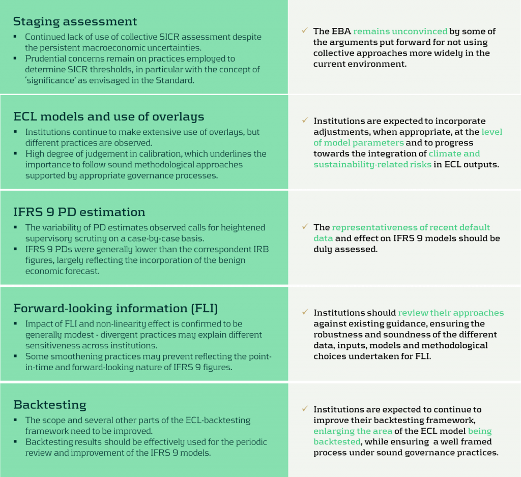
Regulatory view
The EBA published a monitoring report in November 2023 on the current status of the IFRS 9 model landscape (IFRS 9 Monitoring report, EBA (November 2023)). In this report the EBA highlights several takeaways, which are shown in Figure 2. One of these takeaways is the manner in which SICR is modelled at the moment. The EBA is not convinced that non-collective approaches are more suitable than collective approaches. In the results of the survey however, it was shown that most respondents did not indicate SICR as one of the main challenges in their IFRS 9 landscape. This raises the question whether banks in the Netherlands are aware of the EBA’s remark on the current SICR approaches, or whether Dutch banks are outliers when it comes to the SICR modeling approaches.
Furthermore, the report indicates that out-of-model adjustments should be applied on the model parameter level and not on the outcome level. During the roundtable it was discussed that several participants recognize this desire from the regulator, but that they still apply it on the outcome level because the available data only allows for this level. This discrepancy could lead to further scrutiny from the regulator in the near future.
Figure 2: Key takeaways from the IFRS 9 monitoring report (EBA, 2023).
Annual report study
In the Dutch banking market, a variety of modeling practices is observed when it comes to IFRS 9 models for calculating credit loss provisions. Besides gaining insights into these IFRS 9 modeling practices via a survey, annual reports are analyzed to identify potential differences (or similarities) from information that is publicly available.
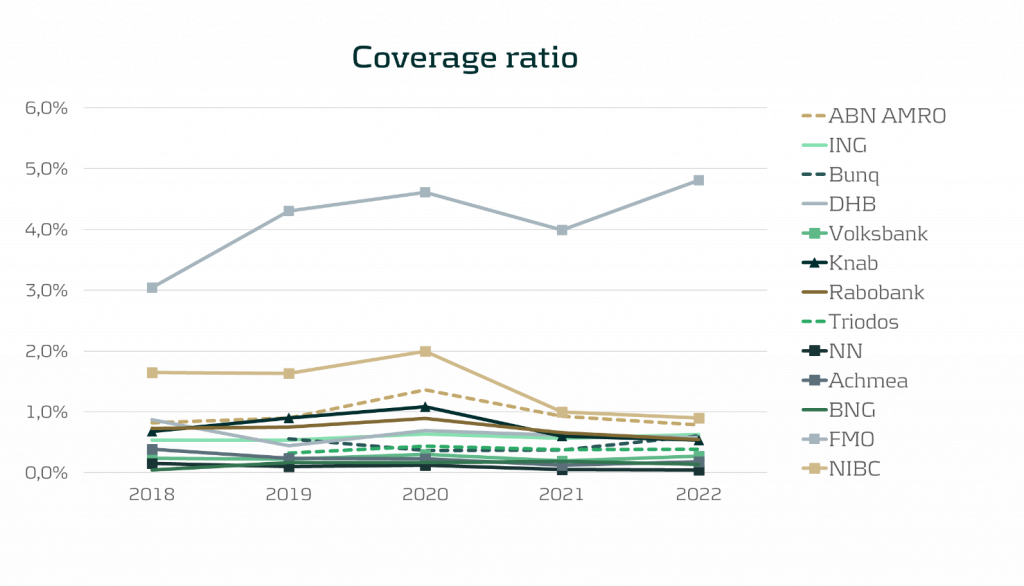
One of the observations from comparing annual reports is that no common level is observed for the Provisioning Coverage Ratio (PCR), i.e. the percentage of funds set aside for covering losses due to bad debts. Characteristics such as portfolio type/composition and loan maturity likely explain these differences. In 2020, almost all banks show an increase in the PCR due to increased allowances in response to the Covid-19 pandemic. Note that this was not necessarily caused by models picking up changing macroeconomic dynamics, but because of model overlays. PCR levels stabilized again in 2021 and 2022.
Figure 3: Coverage ratio over the years 2018 till 2022 . All results were gathered from public annual reports.
Although not all banks report macroeconomic scenario weights in their annual reports, it is worth noting that large differences exist in the scenario weights of banks that do report these figures. Especially weights assigned to the up and down scenarios vary significantly. In 2022, the weight percentage for the base scenario is generally between 40% and 60% (one bank uses a weight of 30%), whereas the weight percentage for the down scenario ranges from 20% to 60%. For the up scenario, percentage weights differ from 2% to 30%. It must be noted that the scenario weights cannot be judged without considering the actual scenario definitions/severity. Nonetheless, the wide variety in scenario weight percentages as well as large differences in the development of these scenario weights over time raises questions on the accuracy of macroeconomic predictions. In addition, it also complicates the comparability of IFRS 9 figures amongst banks.
What can Zanders offer?
We combine deep credit risk modeling expertise with relevant experience in regulation and programming:
- A Risk Advisory Team consisting of 75+ consultants with quantitative backgrounds (e.g. Econometrics and Physics);
- Strong knowledge of IFRS 9 models and developments in the IFRS 9 landscape;
- Extensive experience with calibration, implementation and validation of IFRS 9 models;
- We offer ready-to-use Expected Credit Loss models, Credit Risk Academy modules and expert sessions that can be tailored to the needs of your organization.
Interested to learn more? Contact Kasper Wijshoff or Michiel Harmsen for questions on IFRS 9.


EBA publishes recommendations how to include E&S risks in the prudential framework for banks and insurers.
In October 2023, the European Banking Authority (EBA) published a report[1] with recommendations for enhancements to the Pillar 1 prudential framework to reflect environmental and social (E&S) risks, distinguishing between actions to be taken in the short term and in the medium to long term. The short-term actions are to be taken into account over the next three years as part of the implementation of the revised Capital Requirements Regulation and Capital Requirements Directive (CRR3/CRD6).
The EBA report follows a discussion paper on the same topic from May 2022[2], on which it solicited input from the financial industry. In this note, we provide an overview of the recommended actions by the EBA that relate to the prudential framework for banks. The EBA report also contains recommended actions for the prudential framework applying to investment firms, but these are not addressed here.
If the EBA’s recommendations are implemented in the prudential framework, in our view the most immediate implications for banks would be:
- When using external ratings to determine own fund requirements for credit risk under the standardized approach (SA) of Pillar 1, ensure that E&S risks are explicitly considered when evaluating the appropriateness of the external ratings as part of the due diligence requirements.
- When calculating own fund requirements for credit risk under the internal-ratings-based (IRB) approach, embed E&S risks in the rating assignment, risk quantification (for example through a margin of conservatism or the downturn component) and/or expert judgment and overrides.
- To assess E&S risks at a borrower level, establish a process to obtain and update material E&S-related information on the borrowers’ financial condition and credit facility characteristics, as part of due diligence during onboarding and ongoing monitoring of the borrowers’ risk profile.
- For IRB banks, embed E&S risks in the credit risk stress testing programs.
- Ensure that E&S risks are considered in the valuation of collateral, specifically for financial and real estate collateral.
- For market risk, embed environmental risks in trading book risk appetite, internal trading limits and the new product approval process. Furthermore, for banks aiming to use the internal model approach (IMA) of the Fundamental Review of the Trading Book (FRTB) regulation, environmental risks need to be considered in their stress testing program.
- For operational risk, identify whether E&S risks constitute triggers of operational risk losses.
We note that many of these implications align with the ECB’s expectations in the ECB Guide on climate-related and environmental risks[3].
Background
The EBA report considers both environmental and social risks, which the EBA characterizes as follows:
- As drivers of environmental risks, EBA distinguishes physical and transition (climate) risks. It does not explicitly refer in the report to other environmental risks, such as a loss of biodiversity or pollution, but in an earlier report the EBA considered these as part of chronic physical risks[4].
- EBA considers social factors to be related to the rights, well-being and interests of people and communities, including factors such as decent work, adequate living standards, inclusive and sustainable communities and societies, and human rights. As drivers of social risks, EBA distinguishes environmental factors (as materialization of physical and transition risks may change living standards and the labor market and increase social tensions, for example) as well as changes in policies and market sentiment. These may in part be driven by actions taken to meet the United Nation’s sustainable development goals (SDGs) in 2030.
In line with the ECB Guide on climate-related and environmental risks[5], the EBA does not view E&S risks as stand-alone risks, but as drivers of traditional banking risks. This is depicted in Figure 1. The report considers the impact on credit, market, operational, liquidity and concentration risks and reviews to what extent E&S risks can be reflected in capital buffers and the macro-prudential framework. It does not explicitly consider the securitization framework, although this will be implicitly affected by impacts on credit risk. The EBA does not see an impact of E&S risks on the (risk-insensitive) leverage ratio, and therefore does not consider it in the report.
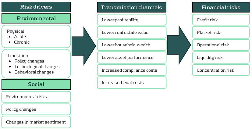
Figure 1: Examples of transmission channels for environmental and social risks (source: EBA).
The EBA notes that the Pillar 1 framework has been designed to capture the possible financial impact of cyclical economic fluctuations, but not to capture the manifestation of long-term environmental risks. It is therefore important to keep the main principles that form the basis of the prudential framework in mind when contemplating adjustments to reflect E&S risks in the prudential framework. The main principles as highlighted by the EBA are summarized below.
Main principles of the prudential framework and the relation to the horizon for E&S risks
With repect to the framework in general:
- Own fund requirements are intended to cover potential unexpected losses. In contrast, expected losses are directly deducted from own funds, and are generally captured in the accounting rules through provisions, impairments, write-downs and appropriate valuation of assets.
- The purpose of own fund requirements is to ensure resilience of an institution to unexpected adverse circumstances, before appropriate mitigating actions and strategy adjustments can be implemented. Therefore, environmental factors that can affect institutions in the short to medium term are expected to be reflected in the prudential framework. However, for those with an impact in the longer term, institutions are expected to take appropriate mitigating actions in their strategy.
- The high confidence level used in the Pillar 1 framework to protect institutions from risks over the short to medium horizon may no longer be achievable and appropriate if longer horizons would be considered.
- To the extent that institutions are exposed to E&S risks in relation to their specific strategy and business model, coverage of these risks in the Pillar 2 own-fund requirements instead of Pillar 1 could be appropriate. In addition, reflection of these risks in the Pillar 2 guidance for stress testing may be considered.
With respect to the internal-ratings-based (IRB) approach for credit risk:
- The Probability of Default (PD) represents a one-year default probability, which is required to be calibrated based on long-run average (‘through-the-cycle’) default rates. As such, longer-term risk characteristics of the obligor may be taken into account.
- The Credit Conversion Factor (CCF) as an estimate of potential additional drawdowns before default naturally relates to the one-year time horizon for the PD, but is expected to reflect the situation of an economic downturn.
- The time horizon for the Loss Given Default (LGD) extends to the full maturity of the exposure and/or the collection process and its calibration is also expected to reflect the situation of an economic downturn.
In the following sections we summarize the EBA recommendations by risk type.
Credit risk
The recommendations of the EBA largely put the burden on financial institutions to take E&S risks into account in the inputs for the existing Pillar 1 framework and/or to apply conservatism or overrides to the outputs. It does not recommend to include explicit E&S risk-related elements in the determination of risk weights for rated and unrated exposures in the SA or in the risk-weight formulas of the IRB. The main reasons for not doing so are that it is not clear what common and objective E&S-related factors should be used as input, what the proper functional form would be, a lack of evidence on which the size of an adjustment could be based so that it results in proper risk differentiation, and the risk of double counting with the reflection of E&S risks in the inputs to the existing own funds calculations under Pillar 1 (external ratings in the SA and PD, LGD and CCF in the case of IRB). However, the EBA will continue to evaluate this possibility in the medium to long term. The EBA also does not recommend introducing an environment-related adjustment factor to the risk weights resulting from the existing Pillar 1 framework[6].
Recommended actions for credit risk
| Short term |
- SA) The EBA encourages rating agencies to integrate environmental and social factors as drivers in the external credit risk assessments and to provide enhanced disclosures and transparency about the rating methodologies.
- (SA) Financial institutions to explicitly consider environmental factors in the due diligence that they are required to perform when using external credit risk assessments.
- (IRB) Financial institutions to reflect E&S risks in the rating assignment, risk quantification (for example through a margin of conservatism or the downturn component) and/or expert judgment and overrides, without affecting the overall performance of the rating system. In this context:
- Quantification of risks must be based on sufficient and reliable observations;
- Overrides should be for specific, individual cases where the institution believes there is material exposure to E&S risks but it has insufficient information to quantify it. Such overrides need to be regularly assessed and challenged;
- If an institution derives PDs for internal rating grades by a mapping to a scale from a credit rating institution, it needs to consider whether the default rates associated with the external scale reflect material E&S risks.
- To assess E&S risks at a borrower level, institutions need to have a process to obtain and update material E&S-related information on the borrowers’ financial condition and on credit facility characteristics, as part of the due diligence during onboarding and ongoing monitoring of borrowers’ risk profile.
- (IRB) Financial institutions to consider E&S risks in their stress testing programs.
- (SA, IRB) Financial institutions to ensure prudent valuation of immovable property collateral, considering climate-related physical and transition risks as well as other environmental risks. The prudent valuation should be considered at origination, re-valuation and during monitoring.
| Medium to long term |
- (SA) Financial institutions to monitor that environmental factors are reflected in financial collateral valuations through market values under Pillar 1 and valuation methodologies under Pillar 2.
- (SA) The EBA to consider whether benefits from the Infrastructure Supporting Factor (ISF) should only be applied to high-quality specialized lending corporate exposures that meet strong environmental standards.
- (SA) The EBA to consider adjusting risk weights, both in general and specifically for those assigned to real estate exposures.
- (IRB) As E&S risks materialize in defaults and loss rates over time, institutions need to redevelop or recalibrate their PD and LGD estimates.
(SA = standardized approach; IRB = Internal-rating-based approach)
Market risk
Within market risk, the EBA sees the main interaction of E&S risks with the equity, credit spread and commodity markets, in which E&S risks may cause additional volatility. In line with the existing regulatory guidance, the EBA expects E&S risks not to be treated as separate risk factors but as drivers of existing risk factors, with the exception of products for which cash flows depend specifically on ESG factors (‘ESG-linked products’).
The EBA does not recommend changes at this point to the standardized approach (SA) and the internal model approach (IMA) under the FRTB regulation, which will come into effect in the EU in 2025. The primary reason is the lack of sufficient evidence on the impact of E&S risks to enable a data driven approach, which forms the basis of the FRTB.
When calculating the expected shortfall (ES) measure under the IMA based on last 12 months' market data, the materialization of E&S risks will automatically be reflected in the market data that is used. When using market data from a stress period, either to calculate ES in the IMA or to calibrate risk factor shocks for the sensitivity-based measure (SbM) at a risk class level in the SA, the reflection of E&S risks will depend on the choice of stress period. To include E&S risks fully in the IMA but avoid overlap with the (partial) presence of E&S risks in historical data, the EBA views the consideration of E&S risks in a separate ‘risk not in the model engine’ (RNIME) add-on as most promising option for the medium to long term, leveraging the framework described in the ECB Guide to internal models[7].
Recommended actions for market risk
| Short term |
- (SA, IMA) Financial institutions to consider environmental risks in relation to their trading book risk appetite, internal trading limits and new product approval.
- (IMA) Financial institutions to consider environmental risk as part of their stress testing program that is required to get internal model approval.
| Medium to long term |
- (SA, IMA) Competent authorities to consider how to treat ESG-linked products for the residual risk add-on in the SA and in the IMA.(SA) The EBA to consider including a dimension for ESG risks in the existing equity and credit spread risk classes, or including a separate environmental risk class.
- (IMA) Financial institutions to consider ESG risks when monitoring risks that are not included in the model, for which the ECB’s RNIME framework could be used as a basis.
(SA = standardized approach; IRB = Internal-rating-based approach)
Operational risk
The EBA notes that various types of operational risks can increase as a result of E&S risks, including damage to physical assets, disruption of business processes and litigation. However, the new standardized approach (SA) for operational risk in the Basel III framework, which will come into effect in the EU in 2025, does not have a forward-looking component – it only considers historical loss experience (besides business indicators). Historical losses are unlikely to fully reflect the potential future impact of E&S risks, but there is as of yet insufficient evidence and data to quantify and consider this in an amendment of the SA.
Recommended actions for operational risk
| Short term |
- Financial institutions to identify whether E&S risks constitute triggers of operational risk losses.
| Medium to long term |
- Following evidence of E&S risk factors to trigger operational risk losses, the EBA to consider whether revisions to the BCBS SA methodology are warranted.
Liquidity risk
The EBA report describes three ways in which E&S risks may affect the liquidity coverage ratio (LCR) calculation. First, liquid assets that are specifically exposed to E&S risks may become less liquid and/or decrease in value. As a consequence, they may no longer satisfy the eligibility criteria for liquid assets. If they still do, then the decrease in market value would reflect the lower liquidity and reduce the LCR. Second, contingent liabilities arising from environmentally harmful investments would need to be included as outflows in the LCR calculation, thereby lowering the LCR. Third, a decrease in credit quality of receivables that are particularly exposed to E&S risks will decrease the inflows that can be taken into account in the LCR calculation. The EBA concludes that the existing LCR framework can capture the impact of E&S risks on the definition of liquid assets, outflows and inflows, so that no amendments are needed.
Regarding the existing framework for the net stable funding ratio (NSFR), the EBA notes that a reduction in the creditworthiness and/or liquidity of loans and securities exposed to E&S risks would lead to a higher requirement for stable funding and thereby negatively impact the NSFR. In this way, the existing NSFR framework can capture the impact of E&S risks on the definition of stable assets.
In summary, the EBA does not propose changes to the LCR and NSFR frameworks in relation to E&S risks. In case of excessive exposure to E&S risks for individual institutions, it notes that supervisors can set specific liquidity or funding requirements as part of the Pillar 2 framework for LCR and NSFR.
Concentration risk
The SA and IRB of the Pillar 1 framework for credit risk assume that a bank’s loan portfolio has full diversification of name-specific (idiosyncratic) risk and is well diversified across sectors and geographies. Because of these assumptions, the framework is not able to capture concentration risks, including those arising from E&S risks. In the current framework, single-name concentration risk is separately captured in Pillar 1 using the large exposure regime. Sector and geographic concentrations are considered in the SREP process under Pillar 2.
Recommended actions for concentration risk
| Short term |
- The EBA to develop a definition of environment-related concentration risk as well as exposure-based metrics for its quantification (e.g., ratio of exposures sensitive to a given environmental risk driver in a specific geographical area or in a specific industry sector over total exposures, total capital or RWA). These metrics will be part of supervisory reporting and, when relevant, external disclosure. In addition, they should be considered as part of Pillar 2 under SREP and/or supplement Pillar 3 disclosures on ESG risks.The EBA does not recommend to change the existing large exposure regime.
| Medium to long term |
- Based on the experience obtained with initial environment-related concentration risk metrics and quantification, the EBA may consider enhanced metrics and the appropriateness to introduce it in the Pillar 1 framework.
- This would entail the design and calibration of possible limits and thresholds, add-ons or buffers, as well as the specification of possible consequences if there are breaches.
Capital buffers and macroprudential framework
An alternative to amending the calculation of capital requirements to capture E&S risks in the prudential framework would be to increase the minimum required level of capital and/or to implement ‘borrower-based measures’ (BMM). Such BMMs aim to prevent a build-up of risk concentrations, for example by setting upper bounds on loan-to-value or loan-to-income for mortgage lending. Of the various possibilities, the EBA deems the use of a systemic risk capital buffer as the most suitable, although a double counting with the inclusion of E&S risks in the calculation of capital requirements under Pillar 1 and 2 needs to be avoided.
Recommended actions for capital buffers and macroprudential framework
| Short term |
- The EBA to asses changes to the guidelines on the appropriate subsets of sectoral exposures to which a systematic risk buffer may be applied.
| Medium to long term |
- The EBA to coordinate with other ongoing initiatives and assess the most appropriate adjustments.
Conclusion
The EBA considers E&S risks as a new source of systemic risk, which may not be adequately captured in the existing prudential framework. At the same time, the EBA recognizes the challenges in assessing the impact of these risks on regulatory metrics. The challenges range from a lack of granular and comparable data, varying definitions of what is environmentally and socially sustainable, historic data not being representative of what can be expected in the future, to the high uncertainty about the probability of future materialization of E&S risks. Moreover, the time horizon considered in the existing Pillar 1 framework is much shorter than the long horizon over which environmental risks are likely to fully materialize, with an exception of short-term acute physical and transition risks.
Against this background, the EBA does not recommend concrete quantitative adjustments to the existing Pillar 1 framework at this point. Nonetheless, it does expect financial institutions to take E&S risks into account in the inputs to the existing Pillar 1 framework or to apply overrides based on expert judgment. The EBA further proposes actions that should provide more clarity over time about the drivers and materiality of E&S risks. In due time, this can provide the basis for quantitative amendments to the Pillar 1 framework.
If you are interested to discuss this topic in more detail or would like support to embed E&S risks in your organization, please contact Pieter Klaassen at [email protected] or +41 78 652 5505.
[1]EBA (2023), Report on the role of environmental and social risks in the prudential framework (link), October.
[2] EBA (2022), Discussion paper on the role of environmental risks in the prudential framework (link), May. For a summary, see the article (link) on the Zanders website.
[3] ECB (2020), Guide on climate-related and environmental risks (link), November.
[4] See section 2.3.2 in EBA (2021), Report on management and supervision of ESG risks for credit institutions and investment firms (link), June.
[5] ECB (2020), Guide on climate-related and environmental risks (link), November.
[6] In the current EU Pillar 1 framework, adjustments are included that result in lower risk weights for small- and medium-sized enterprises (SME) and infrastructure lending. As the EBA notes, these adjustments are not risk-based but have been included in the EU to support lending to SMEs and for infrastructure projects.
One of the main goals of the European Banking Authority (EBA) is to promote supervisory convergence across the European Union regarding supervisory practices. To further the convergence of these supervisory practices the EBA annually outlines key areas of supervisory attention in its European Supervisory Examination Programme (ESEP). On 19 October 2023, the EBA announced the primary focus points for 2024.
Liquidity and funding risk
While European banks generally have sufficient liquidity, there are potential challenges on the horizon. Recent events, including bank failures in the United States and the issues with Credit Suisse, have underscored the importance for banks to have a framework in place that allows a quick response to market volatility and changes in liquidity.
Several factors contribute to these challenges, such as the end of funding programs (i.e. quantitative easing and the TLTRO program), changes in market interest rates, and evolving depositor behavior. The EBA stresses it's not just about meeting regulatory requirements; banks are urged to manage liquidity proactively, maintain reasonable liquidity buffers beyond regulatory mandates, diversify their funding sources, and adapt to changing market dynamics.
The EBA also stresses that the role of social media in relation to the financial markets cannot be underestimated. Banks are encouraged to incorporate social media sentiment into their stress-testing frameworks and develop strategies to counter the impact of negative social media news on deposit withdrawals or market funding stability.
Supervisory authorities should assess institutions’ liquidity risk, funding profiles, and their readiness to deal with wholesale/retail counterparties and funding concentrations. They should also scrutinize banks’ internal liquidity adequacy assessment processes (ILAAP) and their ability to sell securities under different market conditions. Relevant to the increased scrutiny of liquidity and funding risk are the revised technical standards on supervisory reporting on liquidity, published in the summer of 2023 (EBA, June 2023).
Interest rate risk and hedging
The transition from an era of persistently low or even negative interest rates to a period of rising rates and persistent inflation is a major concern for banks in 2024. While the initial impact on net interest margins may be positive, banks face challenges in managing interest rate risk effectively.
Supervisors are tasked with assessing whether banks have suitable organizational frameworks for managing interest rate risk. This includes examining responsibilities at the management level and ensuring that senior management is implementing effective interest rate risk strategies. Moreover, supervisors should evaluate how changes in interest rates may impact an institution’s Net Interest Income (NII) and Economic Value of Equity (EVE). This involves examining assumptions about customers’ behavior, particularly in the context of deposit funding in the digital age.
Interest rate risk and liquidity and funding risk are closely linked, and supervisors are encouraged to consider these links in their assessments, reflecting the interconnected nature of these topics. The new guidelines on IRRBB and CSRBB (EBA, July 2023) emphasize this interconnectedness. It underscores the necessity for financial institutions and regulatory bodies alike to adopt a holistic approach, recognizing that addressing one risk may have cascading effects on others.
The EBA has announced a data collection scheme regarding IRRBB data of financial institutions, highlighting the priority the EBA gives to IRRBB. The data collection exercise is based on the newly published implementing technical standards (ITS) for IRRBB and has a March 2023 deadline. The collection of the IRRBB data will only apply to those institutions that are already reporting IRRBB to the EBA in the context of the QIS exercise.
Recovery operationalization
Recent financial market events (such as Credit Suisse, SVB) have underscored the importance of being prepared for swift and effective crisis responses. Recovery plans, which banks are required to have in place, must be updated and they must include credible options to restore financial soundness in a timely manner.
Supervisors play a vital role in assessing the adequacy and severity of scenarios in recovery plans. These scenarios must be sufficiently severe to trigger the full range of available recovery options, allowing institutions to demonstrate their capacity to restore business and financial viability in a crisis.
Moreover, the Overall Recovery Capacity (ORC) is a key outcome of recovery planning, providing an indication of the institution’s ability to restore its financial position following a significant downturn. It’s crucial for supervisors to review the adequacy and quality of the ORC, with a focus on liquidity recovery capacity.
To ensure the effectiveness of recovery plans, supervisors should also encourage banks to perform dry-run exercises and assess the suitability of communication arrangements, including faster communication tools like social media.
A strategic imperative
Beyond these key focus areas, the EBA also emphasizes the ongoing relevance of issues such as asset quality, cyber risk, and data security. These challenges remain important in the supervisory landscape, although they are not the main priorities in the coming year.
Thus, in light of the EBA’s aforementioned regulatory priorities for 2024, it is imperative for all financial institutions across the European Union to proactively engage in ensuring the stability and resilience of the banking sector. From a liquidity perspective, it is vital to actively manage your financial institution’s liquidity and anticipate the ripples of market volatility. Moreover, the insights of social media sentiment within your stress-testing frameworks can add vital information. The ability to navigate funding challenges is not just a regulatory requirement; it’s a strategic imperative.
The shift to the current high interest rate environment warrants an assessment of a bank’s organizational readiness for this change. Make sure that your senior management is not only aware of implementing effective interest rate risk strategies but also adept at them. Moreover, scrutinize the impact of changing interest rates on your NII and EVE.
How can Zanders support?
Zanders is a thought leader in the management and modeling of IRRBB. We enable financial institutions to meet their strategic risk goals while achieving regulatory compliance, by offering support from strategy to implementation. In light of the aforementioned regulatory priorities of the EBA, we can support and guide you through these changes in the world of IRRBB with agility and foresight.
Are you interested in IRRBB-related topics? Contact Jaap Karelse, Erik Vijlbrief (Netherlands, Belgium and Nordic countries) or Martijn Wycisk (DACH region) for more information.
EBA, July 2023. Guidelines on IRRBB and CSRBB. s.l.:s.n.
EBA, June 2023. Implementing Technical Standards on supervisory reporting amendments with regards to COREP, asset encumbrance and G-SIIs. s.l.:s.n.
EBA, September 2023. Work Program 2024. s.l.:s.n.

Businesses across the globe invest tens of thousands of dollars in implementing treasury management systems to achieve the accuracy, automation, speed, and reporting they require.
But what happens after implementation, when the project team has packed up and handed over the reins to the employees and support staff?
The first months after a system implementation can be some of the most challenging to a business and its people. Learning a new system is like learning any new skill – it requires time and effort to become familiar with the new ways of working, and to be completely comfortable again performing tasks. Previous processes, even if they were not the most efficient, were no doubt second nature to system users and many would have been experts in working their way through what needed to be done to get accurate results. New, improved processes can initially take longer as the user learns how to step through the unfamiliar system. This is a normal part of adopting a new landscape and can be expected. However, employee frustration is often high during this period, as more mental effort is required to perform day-to-day tasks and avoid errors. And when mistakes are made, it often takes more time to resolve them because the process for doing so is unfamiliar.
High-risk period for the company
With an SAP system, the complexity is often great, given the flexibility and available options that it offers. New users of SAP Treasury Management Software may take on average around 12 – 18 months to feel comfortable enough to perform their day-to-day operations, with minimal errors made. This can be a high-risk period for the company, both in terms of staff retention as well as in the mistakes made. Staff morale can dip due to the changes, frustrations and steep learning curve and errors can be difficult to work through and correct.
In-house support staff are often also still learning the new technology and are generally not able to provide the quick turnaround times required for efficient error management right from the start. When the issue is a critical one, the cost of a slow support cycle can be high, and business reputation may even be at stake.

While the benefits of a new implementation are absolutely worthwhile, businesses need to ensure that they do not underestimate the challenges that arise during the months after a system go-live.
Experts to reduce risks
What we have seen is that especially during the critical post-implementation period – and even long afterward – companies can benefit and reduce risks by having experts at their disposal to offer support, and even additional training. This provides a level of relief to staff as they know that they can reach out to someone who has the knowledge needed to move forward and help them resolve errors effectively.
Noticing these challenges regularly across our clients has led Zanders to set up a dedicated support desk. Our Treasury Technology Support (TTS) service can meet your needs and help reduce the risks faced. While we have a large number of highly skilled SAP professionals as part of the Zanders group, we are not just SAP experts. We have a wide pool of treasury experts with both functional & technical knowledge. This is important because it means we are able to offer support across your entire treasury system landscape. So whether it be your businesses inbound services, the multitude of interfaces that you run, the SAP processes that take place, or the delivery of messages and payments to third parties and customers, the Zanders TTS team can help you. We don’t just offer vendor support, but rather are ready to support and resolve whatever the issue is, at any point in your treasury landscape.
As the leading independent treasury consultancy globally, we can fill the gaps where your company demands it and help to mitigate that key person risk. If you are experiencing these challenges or can see how these risks may impact your business that is already in the midst of a treasury system implementation, contact Warren Epstein for a chat about how we can work together to ensure the long-term success of your system investment.


Early 2023, SAP launched its Digital Currency Hub as a pilot to explore the future of cross-border transactions using crypto or digital currencies.
In this article, we explore this stablecoin payments trial, examine the advantages of digital currencies and how they could provide a matching solution to tackle the hurdles of international transactions.
Cross-border payment challenges
While cross-border payments form an essential part of our globalized economy today, they have their own set of challenges. For example, cross-border payments often involve various intermediaries, such as banks and payment processors, which can result in significantly higher costs compared to domestic payments. The involvement of multiple parties and regulations can lead to longer processing times, often combined with a lack of transparency, making it difficult to track the progress of a transaction. This can lead to uncertainty and potential disputes, especially when dealing with unfamiliar payment systems or intermediaries. Last but not least, organizations must ensure they meet the different regulations and compliance requirements set by different countries, as failure to comply can result in penalties or delays in payment processing.
Advantages of digital currencies
Digital currencies have gained significant interest in recent years and are rapidly adopted, both globally and nationally. The impact of digital currencies on treasury is no longer a question of ‘if’ but ‘when’, as such it is important for treasurers to be prepared. While we address the latest developments, risks and opportunities in a separate article, we will now focus on the role digital currencies can play in cross-border transactions.
The notorious volatility of traditional crypto currencies, which makes them less practical in a business context, has mostly been addressed with the introduction of stablecoins and central bank digital currencies. These offer a relatively stable and safe alternative for fiat currencies and bring some significant benefits.
These digital currencies can eliminate the need for intermediaries such as banks for payment processing. By leveraging blockchain technology, they facilitate direct host-to-host transactions with the benefit of reducing transaction fees and near-instantaneous transactions across borders. Transactions are stored in a distributed ledger which provides a transparent and immutable record and can be leveraged for real-time tracking and auditing of cross-border transactions. Users can have increased visibility into the status and progress of their transactions, reducing disputes and enhancing trust. At a more advanced level, compliance measures such as KYC, KYS or AML can be directly integrated to ensure regulatory compliance.
SAP Digital Currency Hub
Earlier this year, SAP launched its Digital Currency Hub as a pilot to further explore the future of cross-border transactions using crypto or digital currencies. The Digital Currency Hub enables the integration of digital currencies to settle transactions with customers and suppliers. Below we provide a conceptual example of how this can work.
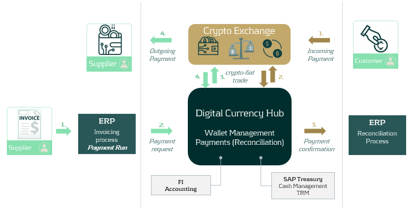
- Received invoices are recorded into the ERP and a payment run is executed.
- The payment request is sent to SAP Digital Currency Hub, which processes the payment and creates an outgoing payment instruction. The payment can also be entered directly in SAP Digital Currency Hub.
- The payment instruction is sent to a crypto exchange, instructing to transfer funds to the wallet of the supplier.
- The funds are received in the supplier’s wallet and the transaction is confirmed back to SAP Digital Currency Hub.
In a second example, we have a customer paying crypto to our wallet:
- The customer pays funds towards our preferred wallet address. Alternatively, a dedicated wallet per customer can be set up to facilitate reconciliation.
- Confirmation of the transaction is sent to SAP Digital Currency Hub. Alternatively, a request for payment can also be sent.
- A confirmation of the transaction is sent to the ERP where the open AR item is managed and reconciled. This can be in the form of a digital bank statement or via the use of an off-chain reference field.
Management of the wallet(s) can be done via custodial services or self-management. There are a few security aspects to consider, on which we recently published an interesting article for those keen to learn more.
While still on the roadmap, SAP Digital Currency Hub can be linked to the more traditional treasury modules such as Cash and Liquidity Management or Treasury and Risk Management. This would allow to integrate digital currency payments into the other treasury activities such as cash management, forecasting or financial risk management.
Conclusion
With the introduction of SAP Digital Currency Hub, there is a valid solution for addressing the current pain points in cross-border transactions. Although the product is still in a pilot phase and further integration with the rest of the ERP and treasury landscape needs to be built, its outlook is promising as it intends to make cross-border payments more streamlined and transparent.

In SAP Treasury, business partners represent counterparties with whom a corporation engages in treasury transactions, including banks, financial institutions, and internal subsidiaries.
Additionally, business partners are essential in SAP for recording information related to securities issues, such as shares and funds.
The SAP Treasury Business Partner (BP) serves as a fundamental treasury master data object, utilized for managing relationships with both external and internal counterparties across a variety of financial transactions; including FX, MM, derivatives, and securities. The BP master data encompasses crucial details such as names, addresses, contact information, bank details, country codes, credit ratings, settlement information, authorizations, withholding tax specifics, and more.
Treasury BPs are integral and mandatory components within other SAP Treasury objects, including financial instruments, cash management, in-house cash, and risk analysis. As a result, the proper design and accurate creation of BPs are pivotal to the successful implementation of SAP Treasury functionality. The creation of BPs represents a critical step in the project implementation plan.
Therefore, we aim to highlight key specifics for professionally designing BPs and maintaining them within the SAP Treasury system. The following section will outline the key focus areas where consultants need to align with business users to ensure the smooth and seamless creation and maintenance of BPs.
Structure of the BPs:
The structure of BPs may vary depending on a corporation's specific requirements. Below is the most common structure of treasury BPs:
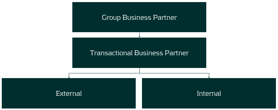
Group BP – represents a parent company, such as the headquarters of a bank group or corporate entity. Typically, this level of BP is not directly involved in trading processes, meaning no deals are created with this BP. Instead, these BPs are used for: a. reflecting credit ratings, b. limiting utilization in the credit risk analyzer, c. reporting purposes, etc.
Transactional BP – represents a direct counterparty used for booking deals. Transactional BPs can be divided into two types:
- External BPs – represent banks, financial institutions, and security issuers.
- Internal BPs – represent subsidiaries of a company.
Naming convention of BPs
It is important to define a naming convention for the different types of BPs, and once defined, it is recommended to adhere to the blueprint design to maintain the integrity of the data in SAP.
Group BP ID: Should have a meaningful ID that most business users can understand. Ideally, the IDs should be of the same length. For example: ABN AMRO Group = ABNAMR or ABNGRP, Citibank Group = CITGRP or CITIBNK.
External BP ID: Should also have a meaningful ID, with the addition of the counterparty's location. For example: ABN AMRO Amsterdam – ABNAMS, Citibank London – CITLON, etc.
Internal BP ID: The main recommendation here is to align the BP ID with the company code number. For example, if the company code of the subsidiary is 1111, then its BP ID should be 1111. However, it is not always possible to follow this simple rule due to the complexity of the ERP and SAP Treasury landscape. Nonetheless, this simple rule can help both business and IT teams find straightforward solutions in SAP Treasury.
The length of the BP IDs should be consistent within each BP type.
Maintenance of Treasury BPs
1. BP Creation:
Business partners are created in SAP using the t-code BP. During the creation process, various details are entered to establish the master data record. This includes basic information such as name, address, contact details, as well as specific financial data such as bank account information, settlement instructions, WHT, authorizations, credit rating, tax residency country, etc.
Consider implementing an automated tool for creating Treasury BPs. We recommend leveraging SAP migration cockpit, SAP scripting, etc. At Zanders we have a pre-developed solution to create complex Treasury BPs which covers both SAP ECC and most recent version of SAP S/4 HANA.
2. BP Amendment:
Regular updates to BP master data are crucial to ensure accuracy. Changes in addresses, contact information, or payment details should be promptly recorded in SAP.
3. BP Release:
Treasury BPs must be validated before use. This validation is carried out in SAP through a release workflow procedure. We highly recommend activating such a release for the creation and amendment of BPs, and nominating a person to release a BP who is not authorized to create/amend a BP.
BP amendments are often carried out by the Back Office or Master Data team, while BP release is handled by a Middle Office officer.
4. BP Hierarchies:
Business partners can have relationships as described, and the system allows for the maintenance of these relationships, ensuring that accurate links are established between various entities involved in financial transactions.
5. Alignment:
During the Treasury BP design phase, it is important to consider that BPs will be utilized by other teams in a form of Vendors, Customers, or Employees. SAP AP/AR/HR teams may apply different conditions to a BP, which can have an impact on Treasury functions. For instance, the HR team may require bank details of employees to be hidden, and this requirement should be reflected in the Treasury BP roles. Additionally, clearing Treasury identification types or making AP/AR reconciliation GL accounts mandatory for Treasury roles could also be necessary.
Transparent and effective communication, as well as clear data ownership, are essential in defining the design of the BPs.
Conclusion
The design and implementation of BPs require expertise and close alignment with treasury business users to meet all requirements and consider other SAP streams.
At Zanders, we have a strong team of experienced SAP consultants who can assist you in designing BP master data, developing tools to create/amend the BPs meeting strict treasury segregation of duties and the clients IT rules and procedures.


As the SWIFT MT-MX migration gains momentum, we are now starting to see more questions from the corporate community around the potential impact of this industry migration.
But the adoption of ISO 20022 XML messaging goes beyond SWIFT’s adoption in the interbank financial messaging space – SWIFT are currently estimating that by 2025, 80% of the RTGS (real time gross settlement) volumes will be ISO 20022 based with all reserve currencies either live or having declared a live date. What this means is that ISO 20022 XML is becoming the global language of payments. In this fourth article in the ISO 20022 series, Zanders experts Eliane Eysackers and Mark Sutton provide some valuable insights around what the version 9 payment message offers the corporate community in terms of richer functionality.
A quick recap on the ISO maintenance process?
So, XML version 9. What we are referencing is the pain.001.001.09 customer credit transfer initiation message from the ISO 2019 annual maintenance release. Now at this point, some people reading this article will be thinking they are currently using XML version 3 and now we talking about XML version 9. The logical question is whether version 9 is the latest message and actually, we expect version 12 to be released in 2024. So whilst ISO has an annual maintenance release process, the financial industry and all the associated key stakeholders will be aligning on the XML version 9 message from the ISO 2019 maintenance release. This version is expected to replace XML version 3 as the de-facto standard in the corporate to bank financial messaging space.
What new functionality is available with the version 9 payment message?
Comparing the current XML version 3 with the latest XML version 9 industry standard, there are a number of new tags/features which make the message design more relevant to the current digital transformation of the payment’s ecosystem. We look at the main changes below:
- Proxy: A new field has been introduced to support a proxy or tokenisation as its sometimes called. The relevance of this field is primarily linked to the new faster payment rails and open banking models, where consumers want to provide a mobile phone number or email address to mask the real bank account details and facilitate the payment transfer. The use of the proxy is becoming more widely used across Asia with the India (Unified Payments Interface) instant payment scheme being the first clearing system to adopt this logic. With the rise of instant clearing systems across the world, we are starting to see a much greater use of proxy, with countries like Australia (NPP), Indonesia (BI-FAST), Malaysia (DuitNow), Singapore (FAST) and Thailand (Promptpay) all adopting this feature.
- The Legal Entity Identifier (LEI): This is a 20-character, alpha-numeric code developed by the ISO. It connects to key reference information that enables clear and unique identification of legal entities participating in financial transactions. Each LEI contains information about an entity’s ownership structure and thus answers the questions of 'who is who’ and ‘who owns whom’. Simply put, the publicly available LEI data pool can be regarded as a global directory, which greatly enhances transparency in the global marketplace. The first country to require the LEI as part of the payment data is India, but the expectation is more local clearing system’s will require this identifier from a compliance perspective.
- Unique End-to-end Transaction Reference (commonly known as a UETR): This is a string of 36 unique characters featured in all payment instruction messages carried over the SWIFT network. UETRs are designed to act as a single source of truth for a payment and provide complete transparency for all parties in a payment chain, as well as enable functionality from SWIFT gpi (global payments innovation)1, such as the payment Tracker.
- Gender neutral term: This new field has been added as a name prefix.
- Requested Execution Date: The requested execution date now includes a data and time option to provide some additional flexibility.
- Structured Address Block: The structured address block has been updated to include the Building Name.
In Summary
Whilst there is no requirement for the corporate community to migrate onto the XML version 9 message, corporate treasury should now have the SWIFT ISO 20022 XML migration on their own radar in addition to understanding the broader global market infrastructure adoption of ISO 20022. This will ensure corporate treasury can make timely and informed decisions around any future migration plan.
Notes:
- SWIFT gpi is a set of standards and rules that enable banks to offer faster, more transparent, and more reliable cross-border payments to their customers.


