EBA Consultation on New CCF Modeling Guidelines

As part of the consultation process, open until 29 October 2025, the credit risk specialists at Zanders share our perspective on the proposed guidelines levering on our extensive expertise in credit risk modeling.

Building on existing EBA guidelines on PD and LGD estimation, the new CCF guideline aims to strengthen consistency across all IRB risk parameters. The proposed guideline provides clearer direction and changes on topics such as:

• Level of modeling: facility-level realized CCFs are required, where aggregation possibilities are limited, and fully drawn facilities are explicitly included in scope.
• Realized CCF: a methodology is provided to determine the CCF based on the level of utilisation.

In addition, the guidelines simplify regulatory expectations compared to the Guidelines on PD and LGD estimation such as:

• Representativeness: model performance outweighs representativeness constraints.
• Risk quantification: the long-run average should be the facility-weighted average of realized CCFs.
• Downturn adjustments: only the extrapolation approach is permitted.
• In-default CCF estimation: the methodology for non-defaulted exposures also applies to defaulted exposures.
• Non-retail exposures: under certain conditions a simplified approach allows using the same CCFs for non-defaulted and defaulted exposures, where estimated drawings for unresolved defaults are omitted.

Recognizing the smaller scope of CCF and data availability compared to PD and LGD, the proposed guidelines introduce a more proportionate and pragmatic approach for CCF estimation.

This article highlights these developments, focusing on the level of modeling, the determination of realized CCF, and the simplified approaches to representativeness, risk quantification, and downturn estimation.

Level of Modeling and Application

Under Article 4(1)(56) of the CRR3, institutions are required to calculate the realized CCF at the level of each individual facility for every default. The EBA’s proposed guidelines enforce this requirement by mandating a separate realized CCF for each facility, allowing exceptions only when several revolving limits stem from related contracts linked through an overarching agreement (i.e. umbrella facility with a shared debt ceiling) and have comparable characteristics.

This represents a clear difference from the flexibility allowed under ECB’s Guide to Internal Models (EGIM) paragraphs 259 and 316, which do not require comparability of characteristics. Under EGIM it is allowed to aggregate at a higher level than the individual facility irrespective of product characteristics, such as aggregation when LGD is estimated at a higher level. The proposed EBA guidelines therefore tightens the existing framework by explicitly prohibiting the aggregation of contracts with very different characteristics.

For institutions, this means developing a deeper understanding of the customer’s product structure and closely monitoring changes in the product mix during the twelve months leading up to a default. A facility is in scope of the CCF model if it contains a revolving contract at the reference date. Contracts that become revolving or non-revolving after a restructuring within the same facility are therefore also included. However, repayments on term loans should not impact the CCF, meaning term loans at the reference date should effectively be excluded. Therefore, institutions must continue to track the exposure as part of the original commitment. This can lead to complex situations, as illustrated below. The brown-highlighted contracts (originating from term loans) are out of scope, while the green-highlighted contracts are in scope. The new contract III is considered in scope because it can be interpreted as an increase in the facility limit.

The realized CCF for this facility is calculated as the difference between the drawn amount at the default date (100 + 50) and the drawn amount at the reference date (50) divided by the undrawn amount at the reference date (50) of the contracts in scope. As a result, the realized CCF is ( (100+50)-50) / (100 – 50) = 200%.

Example:

Moreover, when several facilities are backed by the same collateral, they are often combined into a single recovery account during the recovery process (see example below). In such cases, these facilities can be grouped for LGD. Under the EGIM framework, there was flexibility to also aggregate them for CCF modeling. However, the new guidelines require institutions to precisely allocate outstanding amounts to each specific revolving facility that existed at the reference date. This can create inconsistencies between LGD and CCF modeling and adds complexity to the modeling process. As a result, institutions will need to improve their systems to consistently identify, link, allocate, and manage facilities across their portfolios.

Example:

An obligor has an overarching collateral securing two different facilities I and II. Both facilities consist of revolving off-balance sheet exposures, but have different characteristics. During the recovery process, they are combined into a single recovery account. Therefore, all these facilities are grouped for LGD.

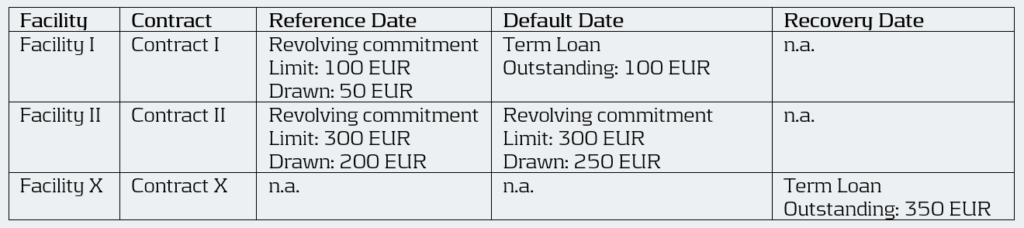
Under EGIM it was permitted to calculate the CCF at the LGD aggregation level, resulting in a realized CCF of ((100 + 250) – (50 + 200)) / ((100+300) – (50+200)) = 66.7%. Under the proposed guidelines, however, the realized CCF must be calculated separately for each facility, giving a CCF of 100% for Facility I (i.e. (100 – 50) / (100 – 50)) and 50% for Facility II (i.e. (250 – 200) / (300 – 200)).

Calculation of Realized CCF

The proposed EBA guidelines introduce two key changes in how institutions determine the realized CCF.

While EGIM paragraph 317 could be interpreted as fully drawn facilities are out of scope, the first change explicitly brings fully drawn revolving commitments into the scope of IRB-CCF modeling, marking another key difference between the two frameworks. EBA’s proposed guidelines now distinguishes between three levels of facility utilization for CCF estimation:

1. Fully drawn facilities.
2. Near-fully drawn facilities, which fall within the so-called Region of Instability (RoI). For example, a facility with a EUR 1000 limit and EUR 995 drawn at the reference date. If an additional EUR 30 is drawn between the reference date and default, the CCF would be: (1020-995)/(1000-995) = 500%.
3. Partially drawn facilities.

The realized CCF is in general determined by the difference in drawn amount at default and the reference date as a percentage of the undrawn amount at the reference date. Since fully drawn facilities have no undrawn part at the reference date, institutions must use an alternative calculation method that expresses the drawn amount at default as a percentage of the committed limit at the reference date. Facilities that are in the RoI, have a very small undrawn amount, which can result in unstable and unreliable realized CCF estimates. Although Basel III describes three possible methods to handle such cases, the guidelines recommend applying the same approach used for fully drawn facilities when predictive accuracy or discriminatory power is limited. They highlight that consistency in applying the chosen approach is essential. Moreover, institutions are expected to define clear thresholds that identify these cases, where it is essential to balance the need to capture outliers without including an excessive number of cases.

The second change concerns the treatment of additional drawings. For retail exposures, institutions retain the flexibility to include additional drawings either in the LGD or in the CCF estimation. For non-retail exposures, additional drawings must still be incorporated into the CCF estimates. In situations where the additional drawings are considered in the CCF all observed drawings should be considered. However, if there are many drawings and repayments, realized CCFs can in practice be very high and LGDs very low (see example below).

Example

The facility has a drawn amount of EUR 100 and a limit of EUR 120, meaning there is an undrawn amount of EUR 20. If the additional drawings would simply be summed, this would lead to a total drawn amount of EUR 60 and a total recovery amount of EUR 160.  As a result, ignoring discounting, this would mean the CCF is EUR 60 / EUR 20 = 300% and the LGD would be ((EUR 100 + EUR 60) – EUR 160) / (EUR 100 + EUR 60) = 0%.

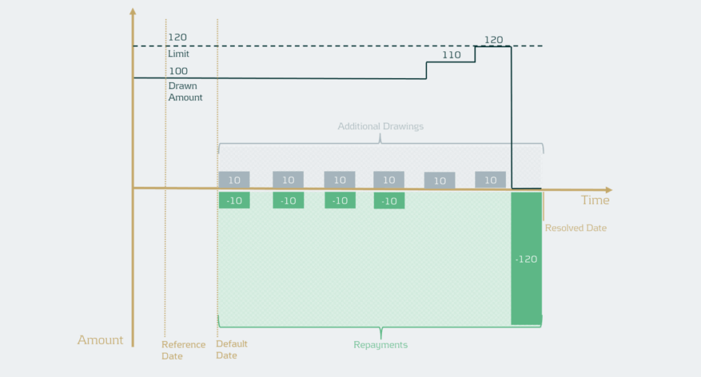
To address this, institutions should now calculate the realized CCF by increasing the drawn amount at default by the positive difference between the highest drawn amount after default and the drawn amount at default. Then the CCF would be (drawn amount at default + additional drawings during default – drawn amount at the reference date) / (limit at reference date – drawn amount at reference date). In the example, the facility has EUR 100 drawn and EUR 20 undrawn at default (and at the reference date for simplicity). The highest drawn amount during default is EUR 120, meaning EUR 20 of additional drawings instead of EUR 60 in the example. Ignoring discounting, this gives a CCF of ((100 + 20) – 100 ) / (120 – 100) =100%. This method uses outstanding balances rather than transaction-level data. It therefore differs from the transaction-based approach typically used in LGD modeling¹. The drawn amounts used in the realized CCF and realized LGD should be consistent, meaning that if an institution currently applies a different method, the LGD model may need to be redeveloped.

Representativeness

While earlier guidelines placed heavy emphasis on ensuring representativeness in the development phase, the proposed guideline focusses on how well the model performs in terms of discriminatory power and homogeneity in rating grades or pools.

However, representativeness remains essential for the data used for developing, testing, and quantifying the CCF models, meaning institutions must still confirm that the data used reflects the characteristics of the application portfolio across different time periods, jurisdictions, and data sources. If the development or testing samples are not representative and this negatively affects model performance or its assessment, they must be redeveloped or adjusted. For the quantification sample, institutions should assess whether any lack of representativeness introduces bias in realized CCFs and apply appropriate adjustments or margins of conservatism where needed, without lowering CCF estimates. Compared to the previous Guidelines on PD and LGD estimation, the new guidelines therefore introduce a simpler approach focused on the performance of the model.

Risk Quantification

Under the EGIM framework, CCF quantification depends on whether the historical observation period is representative of the LRA. If it is, institutions should use the arithmetic average of yearly realized CCFs. If not, adjustments are made to account for underrepresentation or overrepresentation of bad years. The proposed guidelines, however, require a single arithmetic average of all realized CCFs weighted by the number of facilities. It is no longer allowed to use averages based on a subset of observations such as yearly averages. Therefore, potential recalibration is required.

Downturn

The downturn CCF guideline builds on the principles of downturn LGD estimation but introduces several simplifications. The haircut method is removed, as it is considered unsuitable for CCF estimation. Instead, institutions may apply an extrapolation approach at the overall CCF level to capture the direct link between economic factors and CCFs. When no observed or estimated downturn impact is available, a 15%-point add-on is maintained and the105% LGD-cap is removed. Additionally, institutions may apply downturn components estimated for non-defaulted facilities to defaulted ones, eliminating the need for separate downturn estimation and simplifying implementation.

The clarity provided by the new guideline on this topic supports the simplifications aimed to make the framework more pragmatic.

Conclusion

The EBA’s consultation on the new CCF modeling guidelines introduces notable simplifications compared to the previous framework, aiming to enhance consistency across all IRB parameters. While these changes support greater harmonization in credit risk modeling, they also may carry significant implications for institutions, particularly in the areas of level of modeling, realized CCF determination, and long-run average estimation. Adapting effectively to these developments will be essential for maintaining compliance and ensuring robust risk management practices.

The deadline for institutions to submit feedback to the EBA is next week October 29^th 2025. Zanders therefore encourages institutions to evaluate the potential impact on their modeling practices and share insights based on their practical experience.

Reach out to John de Kroon, Dick de Heus, or Louise Schriemer if you are interested in getting a better understanding of what the proposed guidelines mean for your credit risk portfolio.