

The 2025 Swiss Climate Scenarios provide updated estimates of consequences for Switzerland of various global warming scenarios. They cover the likelihood and severity of extreme heat, heavy precipitation, droughts, forest fires, flash floods and thawing permafrost. We summarize the main estimates, highlight the potential economic consequences and discuss ways in which financial institutions can make use of the updated scenarios.
On November 4, MeteoSwiss published updated climate scenarios for Switzerland. The scenarios describe the expected changes in the climate in Switzerland under an increase in global warming by 1.5, 2 and 3 degrees respectively (Global Warming Level (GWL)) compared to the reference period 1991-2020. The timing if and when these GWLs are reached depends on the specific climate scenario considered.
The climate scenarios for Switzerland are anchored in the global climate scenarios that have been included in the sixth and last assessment report of the Intergovernmental Panel on Climate Change (IPCC) from 2022. The three main global scenarios considered are a combination of a Shared Socio-Economic Pathway (SSP) and a Representative Concentration Pathway (RCP):
- “SSP1-2.6” represents a combination of SSP1 and RCP2.6 ("2-degree path with net-zero target achieved by 2050")
- “SSP2-4.5” represents a combination of SSP2 and RCP4.5 (“’Middle ground’ scenario following current and planned measures“)
- “SSP5-8.5” represents a combination of SSP5 and RCP8.5 (“Fossil fuel path without climate protection“)
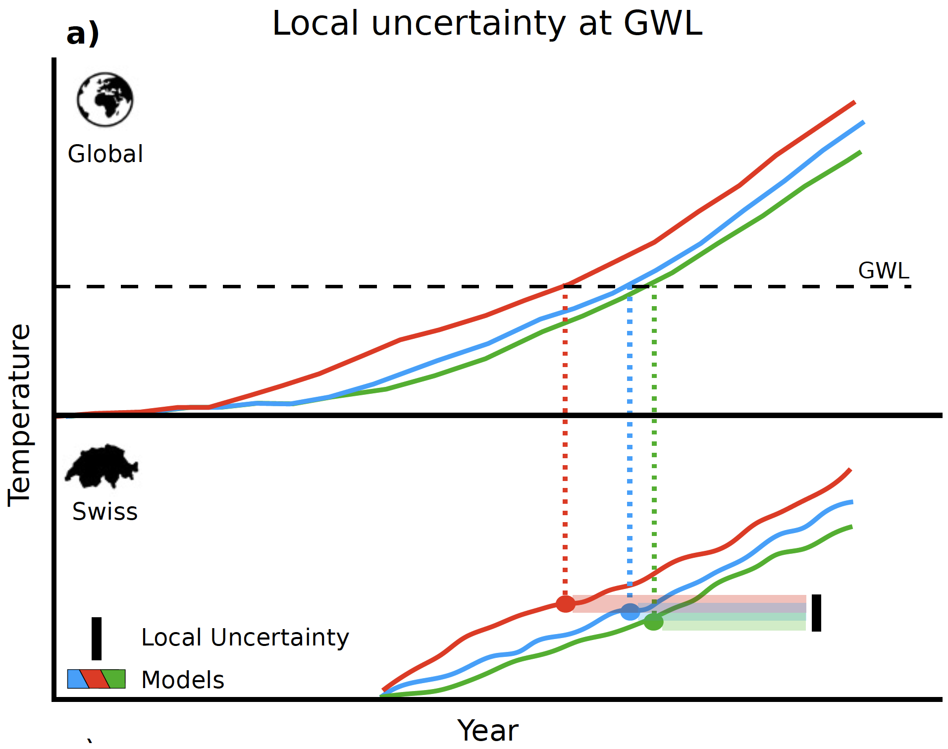
The Figure above depicts the approach taken by MeteoSwiss to assess the consequences for Switzerland at specific GWLs:
- The top part of the Figure (“Global”) shows three global climate scenarios, each of which achieves the depicted GWL at a different point in time.
- MeteoSwiss has translated each of the global scenarios to specific scenarios for Switzerland (more than three in fact, but the picture only shows three). These scenarios are shown in the bottom part of the Figure (“Swiss”). It can be seen that the same GWL in the global scenarios corresponds to different warming levels for Switzerland. This leads to a range of possible warming levels in Switzerland for each GWL.
In the next sections, the main expected changes in temperature and precipitation in Switzerland under the different GWLs are considered. Subsequently, the steps needed to use the information about the climate scenarios for a materiality assessment of climate risk are outlined. In addition, an overview is provided of the data that has been made available for the Swiss climate scenarios by MeteoSwiss, which can be used for such a materiality assessment.
1. Changes in temperature
MeteoSwiss estimates that by 2024, the average temperature in Switzerland already increased by 2.9°C compared to pre-industrial times (1871-1900). This is more than double the rise of 1.4°C in average global temperature. The larger rise in Switzerland is partially due to the fact that the temperature above land increases more quickly than above sea.
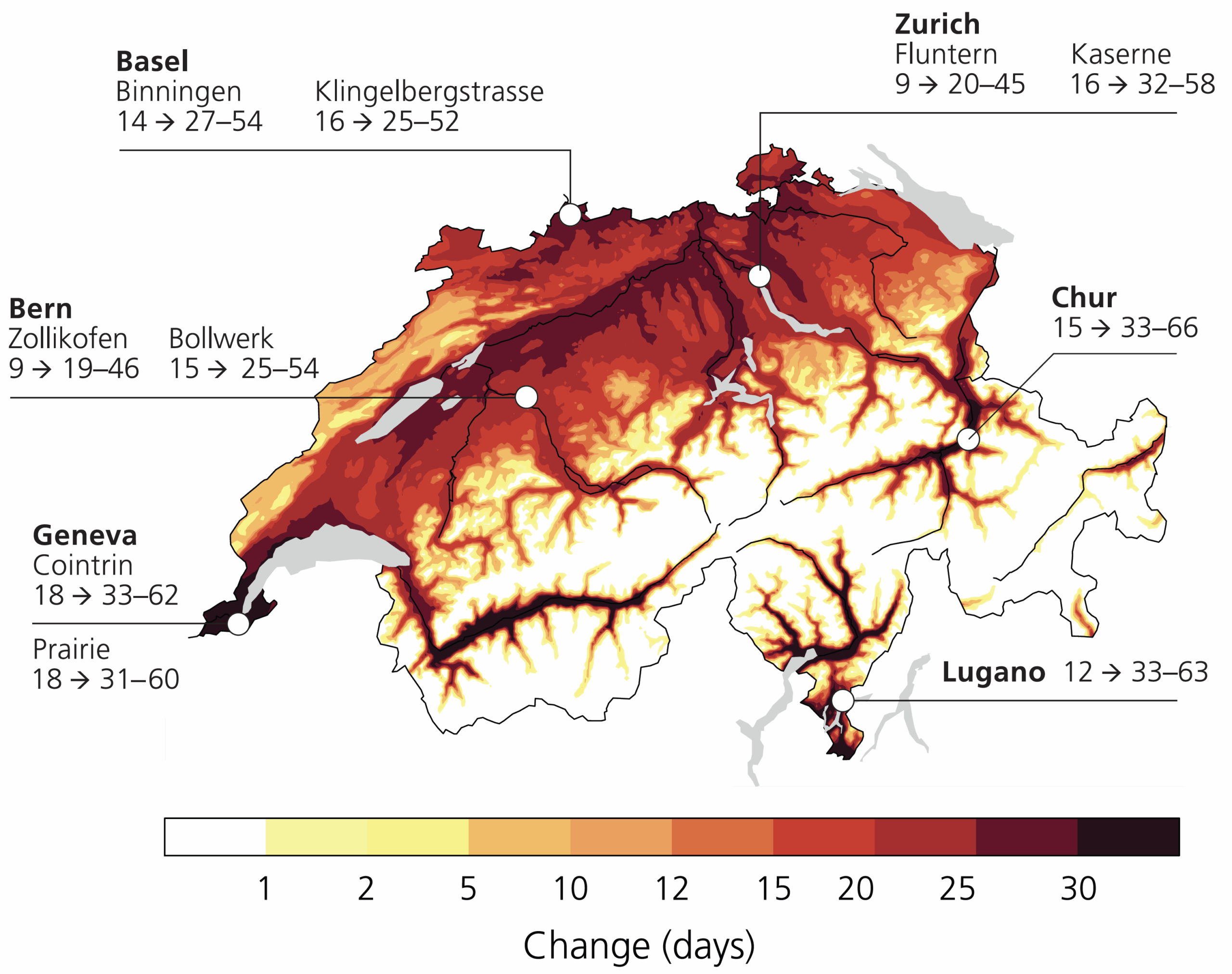
With rising global warming, the number of hot days (>30°C) in Switzerland is expected to roughly triple in a 3-degree world (GWL3.0). The largest impact will be in urban areas, as depicted in the Figure on the right.
In line with this, the average summer temperature as well as extreme temperatures (warmest day and night) will increase.
Potential economic consequences:
- Extreme heat during the day and a lack of cooling at night put strain on the body and affect health. In addition, physical and mental work is made more difficult during heatwaves, with dense urban development exacerbating this. This will affect productivity, lower economic output and may increase costs for cooling work environments.
2. Changes in precipitation
Yearly precipitation is not expected to change in Switzerland with global warming, but summers are expected to get drier and winters are expected to get wetter. Moreover, extreme precipitation (heavy rainfall, hail) is expected to increase in both frequency and intensity, as depicted in the Figure below.
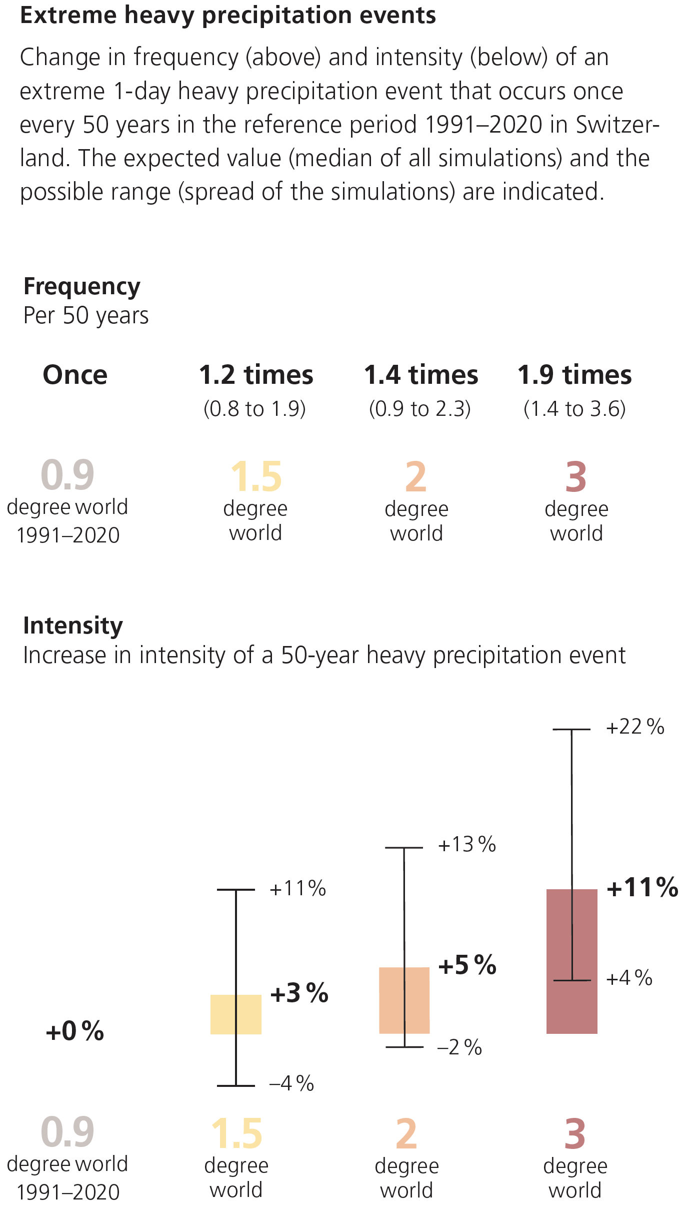
Source: Climate CH2025 – Brochure, MeteoSwiss (link)
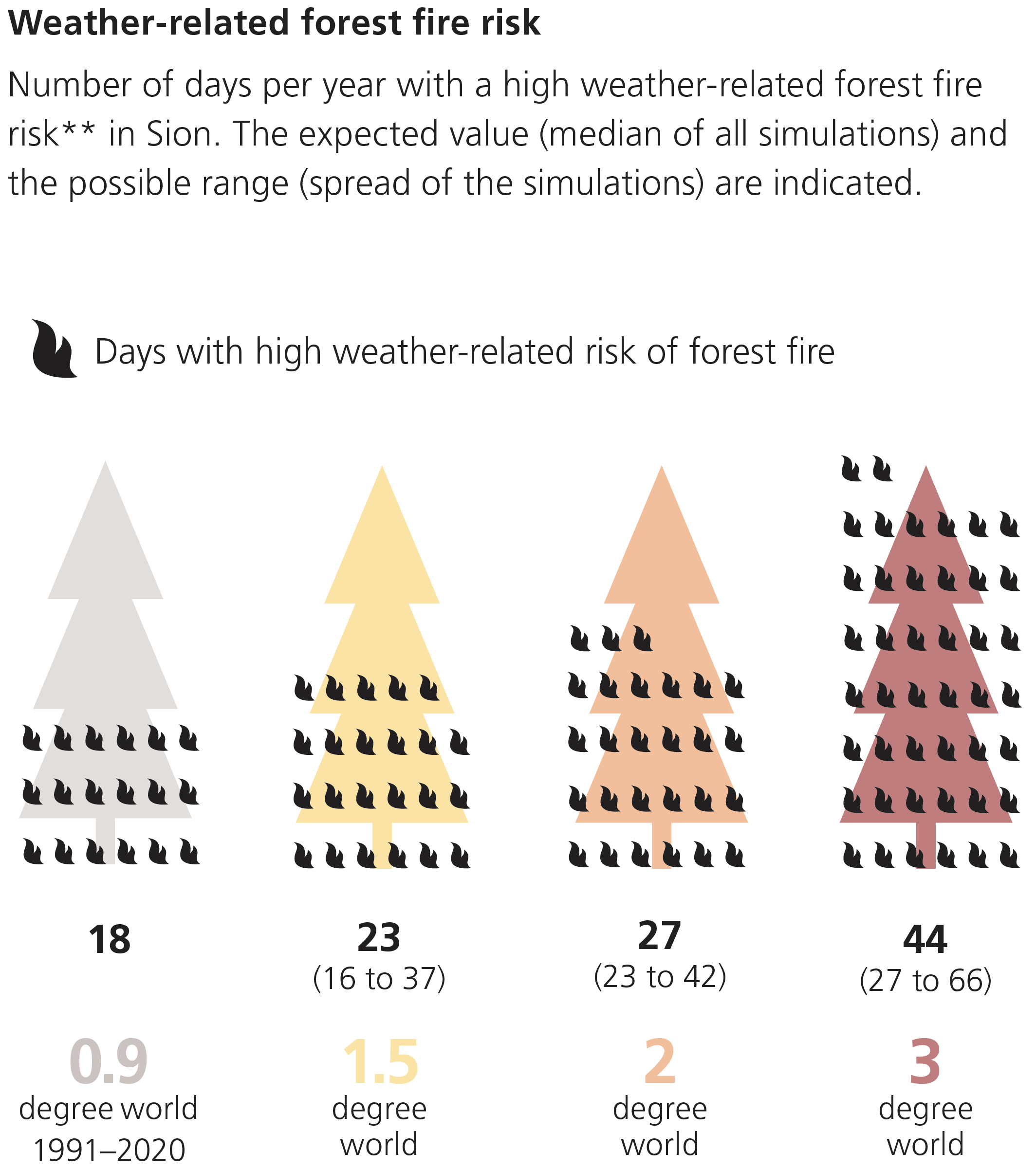
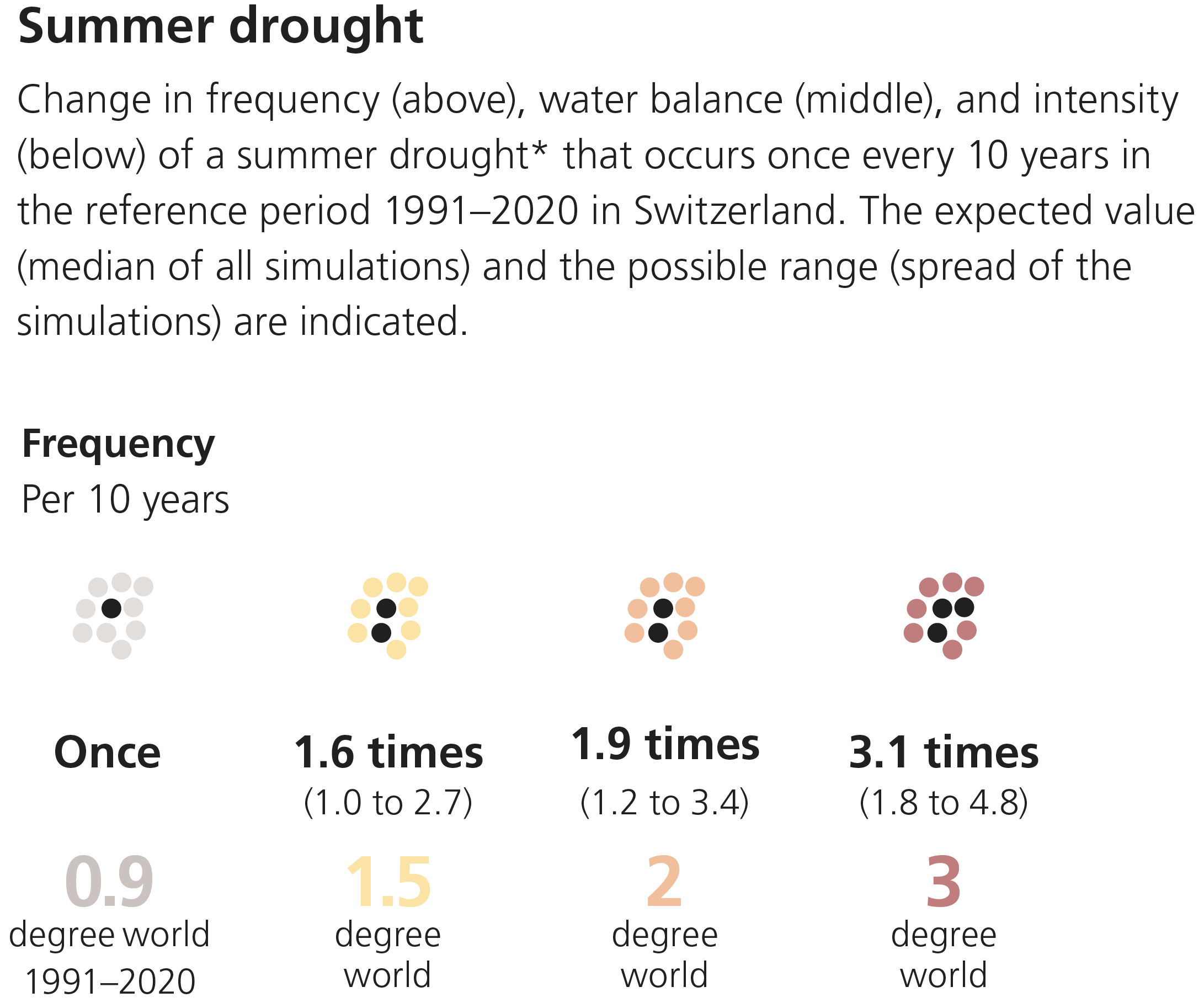
Drier summers lead to an increased risk of forest fires as well as increasing frequency and intensity of droughts, as depicted in the Figures below.
Precipitation in winter will increasingly fall in the form of rain instead of snow as the zero-degree line increases.
Potential economic consequences:
- Sudden flash floods and hail can cause property damage and business interruptions. In addition, they can destroy agricultural crops. This will negatively affect economic output and decrease the value of properties in areas at risk.
- Drought leads to yield losses in agriculture and increased risk of forest fires, causes water shortages in reservoirs and restricts water supply. In addition, drought can intensify and prolong heatwaves. This will negatively affect economic output
- Thawing permafrost and melting glaciers can lead to unstable slopes, and the water cycle may be disrupted. This will affect industries that depend on water (e.g., for cooling). Decreasing snow will also affect winter tourism and associated industry sectors.
3. Estimating financial impacts
For the potential future changes in temperature and precipitation in Switzerland because of global warming, the possible economic consequences have been explored in the sections above. To what extent these are relevant for risk management of a financial institution will depend on the sectors and physical locations of their clients, counterparties and issuers of securities in which they invest.
The general steps taken to perform a materiality assessment for individual clients, counterparties and issuers are:
1. Identify transmission channels through which the impacts of global warming can negatively impact their business.
2. Estimate the financial impact of individual transmission channels.
- As historical data is not representative of what is likely to happen in the future under global warming, a common approach is to use scenario analysis.
- FINMA explicitly expects financial institutions to employ scenario analysis when performing the materiality assessment for nature-related financial risks in its recent circular (link, see our Zanders blog for a summary).
- The Swiss climate scenarios can form a basis for the scenario analysis. However, the climate impacts that have been made available by MeteoSwiss (see Section 4) need to be translated to a financial impact for clients, counterparties and issuers. The impact on both revenues (e.g., lower sales due to business disruptions or lower demand) and costs (e.g., higher costs due to damages or required additional investments) need to considered.
- Mitigating measures such as insurance can be taken into account if they are deemed effective in the scenarios considered.
3. Reflect the estimated financial impact in internal risk metrics, such as credit ratings, collateral values and the value-at-risk of investments.
For companies that are active internationally, or which depend on international supply chains, the exposure of their supply chains and international markets to the impact of global warming also needs to be considered.
4. Swiss climate scenario data
With the publication of the Swiss climate scenarios, MeteoSwiss also makes available detailed scenario data. This data can be viewed through an interactive WebAtlas (link) for combinations of:
- Various temperature and precipitation indicators (listed in the document “Overview of CH2025 climate indicators” (link))
- Reference period (1991-2020) and three future Global Warming Levels (GWL1.5, GWL2.0 and GWL3.0)
- Annual changes as well as seasonal changes (Winter, Spring, Sommer and Autumn)
- Switzerland as a whole, each of five ‘biogeographic’ regions (Jura, Swiss Plateau, Pre-Alps, Alps, and South side of the Alps) as well as individual weather stations
- Three climate scenarios (SSP1-2.6, SSP2-4.5 and SSP5-8.5) over time (2040-2060) (for mean temperature and precipitation only)
The following detailed data can also be accessed directly:
- Historical climate data (daily) at individual Swiss measurement stations since measurement started, covering 169 indicators related to temperature, humidity, precipitation, wind, sunshine, snow, air pressure, evaporation and radiation. (link)
- These data have been ‘homogenized’ for changes in measurement methods over time.
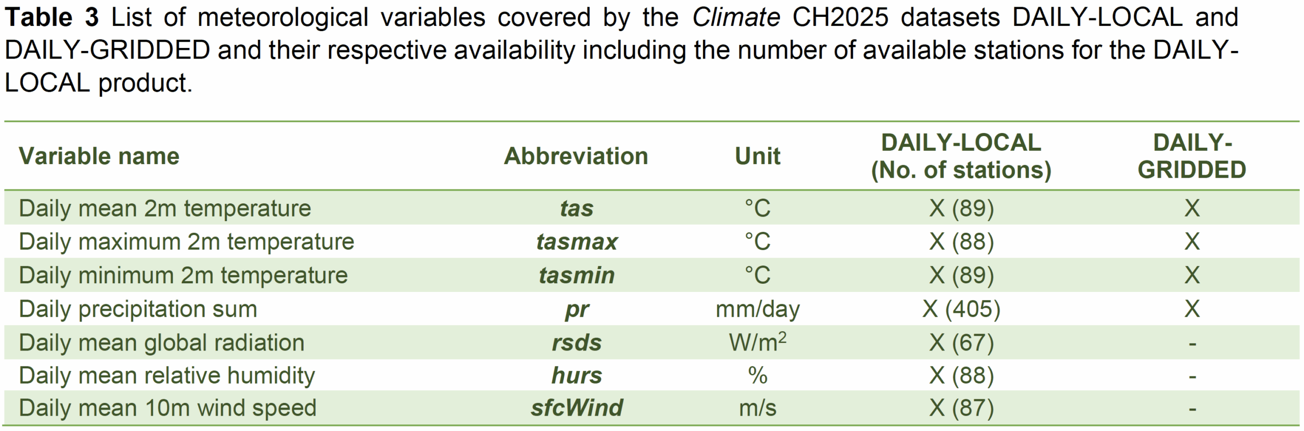
- Scenario forecast data (daily) for different Global Warming Levels (GWL) under different Regional Climate Models (RMC) (link)(link) at
- Individual weather stations (DAILY_LOCAL)
- 1km×1km gridpoints in Switzerland (DAILY-GRIDDED)
Climate variables included in the daily scenario forecasts are shown in the table below.
How Zanders can help
We have supported various banks with the assessment of the materiality of climate risks for their clients, counterparties and investment issuers. With our focus on risk and technology and our strength in applying quantitative approaches, we are particularly well equipped to substantiate a materiality assessment with scenario analysis and the use of data. If you want to learn more, do not hesitate to contact us.

Get climate risk support
Speak to an expert
Machine learning (ML) models have already been around for decades. The exponential growth in computing power and data availability, however, has resulted in many new opportunities for ML models. One possible application is to use them in financial institutions’ risk management. This article gives a brief introduction of ML models, followed by the most promising opportunities for using ML models in financial risk management.
The current trend to operate a ‘data-driven business’ and the fact that regulators are increasingly focused on data quality and data availability, could give an extra impulse to the use of ML models.
ML models
ML models study a dataset and use the knowledge gained to make predictions for other datapoints. An ML model consists of an ML algorithm and one or more hyperparameters. ML algorithms study a dataset to make predictions, where hyperparameters determine the settings of the ML algorithm. The studying of a dataset is known as the training of the ML algorithm. Most ML algorithms have hyperparameters that need to be set by the user prior to the training. The trained algorithm, together with the calibrated set of hyperparameters, form the ML model.
ML models have different forms and shapes, and even more purposes. For selecting an appropriate ML model, a deeper understanding of the various types of ML that are available and how they work is required. Three types of ML can be distinguished:
- Supervised learning.
- Unsupervised learning.
- Semi-supervised learning.
The main difference between these types is the data that is required and the purpose of the model. The data that is fed into an ML model is split into two categories: the features (independent variables) and the labels/targets (dependent variables, for example, to predict a person’s height – label/target – it could be useful to look at the features: age, sex, and weight). Some types of machine learning models need both as an input, while others only require features. Each of the three types of machine learning is shortly introduced below.
Supervised learning
Supervised learning is the training of an ML algorithm on a dataset where both the features and the labels are available. The ML algorithm uses the features and the labels as an input to map the connection between features and labels. When the model is trained, labels can be generated by the model by only providing the features. A mapping function is used to provide the label belonging to the features. The performance of the model is assessed by comparing the label that the model provides with the actual label.
Unsupervised learning
In unsupervised learning there is no dependent variable (or label) in the dataset. Unsupervised ML algorithms search for patterns within a dataset. The algorithm links certain observations to others by looking at similar features. This makes an unsupervised learning algorithm suitable for, among other tasks, clustering (i.e. the task of dividing a dataset into subsets). This is done in such a manner that an observation within a group is more like other observations within the subset than an observation that is not in the same group. A disadvantage of unsupervised learning is that the model is (often) a black box.
Semi-supervised learning
Semi-supervised learning uses a combination of labeled and unlabeled data. It is common that the dataset used for semi-supervised learning consist of mostly unlabeled data. Manually labeling all the data within a dataset can be very time consuming and semi-supervised learning offers a solution for this problem. With semi-supervised learning a small, labeled subset is used to make a better prediction for the complete data set.
The training of a semi-supervised learning algorithm consists of two steps. To label the unlabeled observations from the original dataset, the complete set is first clustered using unsupervised learning. The clusters that are formed are then labeled by the algorithm, based on their originally labeled parts. The resulting fully labeled data set is used to train a supervised ML algorithm. The downside of semi-supervised learning is that it is not certain the labels are 100% correct.
Setting up the model
In most ML implementations, the data gathering, integration and pre-processing usually takes more time than the actual training of the algorithm. It is an iterative process of training a model, evaluating the results, modifying hyperparameters and repeating, rather than just a single process of data preparation and training. After the training is performed and the hyperparameters have been calibrated, the ML model is ready to make predictions.
Machine learning in financial risk management
ML can add value to financial risk management applications, but the type of model should suit the problem and the available data. For some applications, like challenger models, it is not required to completely explain the model you are using. This makes, for example, an unsupervised black box model suitable as a challenger model. In other cases, explainability of model results is a critical condition while choosing an ML model. Here, it might not be suitable to use a black box model.
In the next section we present some examples where ML models can be of added value in financial risk management.
Data quality analysis
All modeling challenges start with data. In line with the ‘garbage in, garbage out’ maxim, if the quality of a dataset is insufficient then an ML model will also not perform well. It is quite common that during the development of an ML model, a lot of time is spent on improving the data quality. As ML algorithms learn directly from the data, the performance of the resulting model will increase if the data quality increases. ML can be used to improve data quality before this data is used for modeling. For example, the data quality can be improved by removing/replacing outliers and replacing missing values with likely alternatives.
An example of insufficient data quality is the presence of large or numerous outliers. An outlier is an observation that significantly deviates from the other observations in the data, which might indicate it is incorrect. Outlier detection can easily be performed by a data scientist for univariate outliers, but multivariate outliers are a lot harder to identify. When outliers have been detected, or if there are missing values in a dataset, it might be useful to substitute some of these outliers or impute for missing values. Popular imputation methods are the mean, median or most frequent methods. Another option is to look for more suitable values; and ML techniques could help to improve the data quality here.
Multiple ML models can be combined to improve data quality. First, an ML model can be used to detect outliers, then another model can be used to impute missing data or substitute outliers by a more likely value. The outlier detection can either be done using clustering algorithms or by specialized outlier detection techniques.
Loan approval
A bank’s core business is lending money to consumers and companies. The biggest risk for a bank is the credit risk that a borrower will not be able to fully repay the borrowed amount. Adequate loan approval can minimize this credit risk. To determine whether a bank should provide a loan, it is important to estimate the probability of default for that new loan application.
Established banks already have an extensive record of loans and defaults at their disposal. Together with contract details, this can form a valuable basis for an ML-based loan approval model. Here, the contract characteristics are the features, and the label is the variable indicating if the consumer/company defaulted or not. The features could be extended with other sources of information regarding the borrower.
Supervised learning algorithms can be used to classify the application of the potential borrower as either approved or rejected, based on their probability of a future default on the loan. One of the suitable ML model types would be classification algorithms, which split the dataset into either the ‘default’ or ‘non-default’ category, based on their features.
Challenger models
When there is already a model in place, it can be helpful to challenge this model. The model in use can be compared to a challenger model to evaluate differences in performance. Furthermore, the challenger model can identify possible effects in the data that are not captured yet in the model in use. Such analysis can be performed as a review of the model in use or before taking the model into production as a part of a model validation.
The aim of a challenger model is to challenge the model in use. As it is usually not feasible to design another sophisticated model, mostly simpler models are selected as challenger model. ML models can be useful to create more advanced challenger models within a relatively limited amount of time.
Challenger models do not necessarily have to be explainable, as they will not be used in practice, but only as a comparison for the model in use. This makes all ML models suitable as challenger models, even black box models such as neural networks.
Segmentation
Segmentation concerns dividing a full data set into subsets based on certain characteristics. These subsets are also referred to as segments. Often segmentation is performed to create a model per segment to better capture the segment’s specific behavior. Creating a model per segment can lower the error of the estimations and increase the overall model accuracy, compared to a single model for all segments combined.
Segmentation can, among other uses, be applied in credit rating models, prepayment models and marketing. For these purposes, segmentation is sometimes based on expert judgement and not on a data-driven model. ML models could help to change this and provide quantitative evidence for a segmentation.
There are two approaches in which ML models can be used to create a data-driven segmentation. One approach is that observations can be placed into a certain segment with similar observations based on their features, for example by applying a clustering or classification algorithm. Another approach to segment observations is to evaluate the output of a target variable or label. This approach assumes that observations in the same segment have the same kind of behavior regarding this target variable or label.
In the latter approach, creating a segment itself is not the goal, but optimizing the estimation of the target variable or classifying the right label is. For example, all clients in a segment ‘A’ could be modeled by function ‘a’, where clients in segment ‘B’ would be modeled by function ‘b’. Functions ‘a’ and ‘b’ could be regression models based on the features of the individual clients and/or macro variables that give a prediction for the actual target variable.
Credit scoring
Companies and/or debt instruments can receive a credit rating from a credit rating agency. There are a few well-known rating agencies providing these credit ratings, which reflects their assessment of the probability of default of the company or debt instrument. Besides these rating agencies, financial institutions also use internal credit scoring models to determine a credit score. Credit scores also provide an expectation on the creditworthiness of a company, debt instrument or individual.
Supervised ML models are suitable for credit scoring, as the training of the ML model can be done on historical data. For historical data, the label (‘defaulted’ or ‘not defaulted’) can be observed and extensive financial data (the features) is mostly available. Supervised ML models can be used to determine reliable credit scores in a transparent way as an alternative to traditional credit scoring models. Alternatively, credit scoring models based on ML can also act as challenger models for traditional credit scoring models. In this case, explainability is not a key requirement for the selected ML model.
Conclusion
ML can add value to, or replace, models applied in financial risk management. It can be used in many different model types and in many different manners. A few examples have been provided in this article, but there are many more.
ML models learn directly from the data, but there are still some choices to be made by the model user. The user can select the model type and must determine how to calibrate the hyperparameters. There is no ‘one size fits all’ solution to calibrate a ML model. Therefore, ML is sometimes referred to as an art, rather than a science.
When applying ML models, one should always be careful and understand what is happening ‘under the hood’. As with all modeling activities, every method has its pitfalls. Most ML models will come up with a solution, even if it is suboptimal. Common sense is always required when modeling. In the right hands though, ML can be a powerful tool to improve modeling in financial risk management.
Working with ML models has given us valuable insights (see the box below). Every application of ML led to valuable lessons on what to expect from ML models, when to use them and what the pitfalls are.
Machine learning and Zanders
Zanders already encountered several projects and research questions where ML could be applied. In some cases, the use of ML was indeed beneficial; in other cases, traditional models turned out to be the better solution.
During these projects, most time was spent on data collection and data pre-processing. Based on these experiences, an ML based dataset validation tool was developed. In another case, a model was adapted to handle missing data by using an alternative available feature of the observation.
ML was also used to challenge a Zanders internal credit rating model. This resulted in useful insights on potential model improvements. For example, the ML model provided more insight in variable importance and segmentation. These insights are useful for the further development of Zanders’ credit rating models. Besides the insights what could be done better, the ML model also emphasized the advantages of classical models over the ML-based versions. The ML model was not able to provide more sensible ratings than the traditional credit rating model.
In another case, we investigated whether it would be sensible and feasible to use ML for transaction screening and anomaly detection. The outcome of this project once more highlighted that data is key for ML models. The available data was numerous, but of low quality. Therefore, the used ML models were not able to provide a helpful insight into the payments, or to consistently detect divergent payment behavior on a large scale.
Besides the projects where ML was used to deliver a solution, we investigated the explainability of several ML models. During this process we gained knowledge on techniques to provide more insights into otherwise hardly understandable (black box) models.


