With support for their long-standing hedge accounting models ending in 2025, global asset finance company, DLL, sought a partner capable of not just replicating their existing models but enhancing and futureproofing them – on a tight timeline. To guide the company’s treasury through this critical crossroad, DLL turned to Zanders.
DLL (De Lage Landen) is a global asset finance company headquartered in Eindhoven, the Netherlands, and a wholly owned subsidiary of Rabobank. Operating in more than 25 countries, it delivers leasing and asset-based financing solutions across a variety of industry sectors, including agriculture, construction, energy transition, food, healthcare, industrial, technology, and transportation. With a strong focus on responsible finance, the company supports businesses to access capital, manage risk, and make the transition to more sustainable business models.
Central to the company’s financial infrastructure is its global treasury function, based in Dublin, Ireland. This team manages the liquidity and Treasury risk management needs of the group. The team consists of an experienced group of highly qualified financial services professionals who are dedicated to meeting the treasury needs of DLL, covering everything from cash management to foreign exchange and interest rate hedging.
A critical turning point
A core element of DLL’s risk strategy is the use of interest rate swaps to mitigate exposure to interest rate volatility. Given the size and complexity of its global lending portfolio and the direct impact that interest rate movements can have on company earnings, these instruments are essential for maintaining financial stability and predictability.
“We have two large portfolios – euro interest rate swaps and US dollar interest rate swaps,” explains Coyle, Head of Hedge Accounting at DLL. “To mitigate the fair value movements of those swaps, we run macro fair value hedge accounting models in euros and dollars.”
These models allow DLL to align the value of derivatives with the risks they offset. This reduces earnings volatility, provides a transparent view of the company’s risk position, and ensures compliance with accounting standards.
For years, DLL’s hedge accounting models were developed and maintained by a previous provider. Due to regulatory requirements they were no longer allowed to support the models beyond 2025.
Faced with a tight deadline to transition to a new solution, DLL launched a competitive tender process to identify a partner capable of building fair value macro hedge accounting models for both their euro and dollar swap portfolios. To prevent disruption to DLL’s hedge accounting process, replacement models needed to be ready for testing in early 2025, ahead of full deployment a few months later. This challenging timeline relied on delivering a complete, fully tested and operational solution as quickly as possible, rather than following a more gradual, phased approach.
Zanders’ approach stood out because they proposed building a Python-based application from the start – delivering the end product we needed, and within the timeline that we wanted.
Coyle, Head of Hedge Accounting at DLL.

“Another provider suggested an Excel build first, then a Python version later – essentially two separate projects, which would not only take a lot longer but also impacted on the price as well.”
Rapid prototyping and agile development
Once selected in late 2024, Zanders began working on replicating the models. Despite having no access to the original model’s codebase, the Zanders team was able to reverse engineer DLL’s hedge accounting methodology in just a few weeks based.
“They started in December, and by the end of January we had our first models ready for testing,” Coyle recalls.
From February to March, both Zanders and DLL conducted independent back testing using the legacy model as a benchmark to validate outputs. This rigorous comparison helped ensure consistency and build confidence in the new models.
“This gave us comfort that we were on the right road,” Coyle says. “We did find a few things that we wanted to change – such as adding certain risk controls – and the Zanders team was very open to suggestions. These were implemented quickly, and it was a very easy process.”
By the end of March, the new Python-based applications was fully operational, enabling a seamless transition with no disruption to DLL’s interest rate risk strategy.
Faster, simpler, more integrated
While the primary focus of the project was the replication of DLL’s existing models, it ultimately evolved into an opportunity to streamline and modernize the company’s hedge accountancy processes.
“The new model is much quicker,” explains Marais, Treasury Hedge Accountant at DLL. “The old model had features we didn’t really use that slowed down performance. This was a chance to simplify and focus on what we needed.”
One of the most valuable technical gains was improved alignment with DLL’s internal treasury systems.
“With the new model, we are now able to utilize reports from our own treasury system – that was a significant improvement,” says Marais. Previously, the team had to rely on reports from Rabobank systems and model calculations, but the new model directly interfaces with DLL's internal system. “This makes our work process much quicker and more efficient compared to previously,” Marais adds.
Beyond the technical delivery, the project also stood out for the way it was executed. Working under a tight deadline, collaboration between the teams was critical and made a real difference to the overall experience. The DLL team particularly appreciated Zanders’ responsive and collaborative approach.
IT projects can be quite stressful, but this one was remarkably stress-free. That’s a reflection of a robust, collaborative process and great people. If someone asked whether we’d recommend the Zanders team for a project like this, we wouldn’t hesitate.
Coyle, Head of Hedge Accounting at DLL.
Interested in transforming your treasury infrastructure?
Whether you're navigating regulatory change, replacing legacy models, or looking to gain deeper insights into your risk exposure, Zanders combines advanced modeling with deep industry expertise to deliver accurate and audit-ready valuations.
Find out more about how Zanders can support your treasury and risk management transformation.

Ready to transform your treasury infrastructure?
Contact us
Emergence of Artificial Intelligence and Machine Learning
The rise of ChatGPT has brought generative artificial intelligence (GenAI) into the mainstream, accelerating adoption across industries ranging from healthcare to banking. The pace at which (Gen)AI is being used is outpacing prior technological advances, putting pressure on individuals and companies to adapt their ways of working to this new technology. While GenAI uses data to create new content, traditional AI is typically designed to perform specific tasks such as making predictions or classifications. Both approaches are built on complex machine learning (ML) models which, when applied correctly, can be highly effective even on a stand-alone basis.
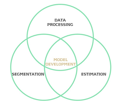
Figure 1: Model development steps
Though ML techniques are known for their accuracy, a major challenge lies in their complexity and limited interpretability. Unlocking the full potential of ML requires not only technical expertise, but also deep domain knowledge. Asset and Liability Management (ALM) departments can benefit from ML, for example in the area of behavioral modeling. In this article, we explore the application of ML in prepayment modeling (data processing, segmentation, estimation) based on research conducted at a Dutch bank. The findings demonstrate how ML can improve the accuracy of prepayment models, leading to better cashflow forecasts and, consequently, a more accurate hedge. By building ML capabilities in this context, ALM teams can play a key role in shaping the future of behavioral modeling throughout the whole model development process.
Prepayment Modeling and Machine Learning
Prepayment risk is a critical concern for financial institutions, particularly in the mortgage sector, where borrowers have the option to repay (a part of) their loans earlier than contractually agreed. While prepayments can be beneficial for borrowers (allowing them to refinance at lower interest rates or reduce their debt obligations) they present several challenges for financial institutions. Uncertainty in prepayment behaviour makes it harder to predict the duration mismatch and the corresponding interest rate hedge.
Effective prepayment modeling by accurately forecasting borrower behavior is crucial for financial institutions seeking to manage interest rate risks. Improved forecasting enables institutions to better anticipate cash flow fluctuations and implement more robust hedging strategies. To facilitate the modeling, data is segmented based on similar prepayment characteristics. This segmentation is often based on expert judgment and extensive data analysis, accounting for factors like loan age, interest rate, type, and borrower characteristics. Each segment is then analyzed through tailored prepayment models, such as a logistic regression or survival models.1
ML techniques offer significant potential to enhance segmentation and estimation in prepayment modeling. In rapidly changing interest rate environments, traditional models often struggle to accurately capture borrower behavior that deviates from conventional financial logic. In contrast, ML models can detect complex, non-linear patterns and adapt to changing behaviour, improving predictive accuracy by uncovering hidden relationships. Investigating such relationships becomes particularly relevant when borrower actions undermine traditional assumptions, as was the case in early 2021, when interest rates began to rise but prepayment rates did not decline immediately.
Real-world application
In collaboration with a Dutch bank, we conducted research on the application of ML in prepayment modeling within the Dutch mortgage market. The applications include data processing, segmentation, and estimation followed by an interpretation of the results with the use of ML specific interpretability metrics. Despite being constrained by limited computational power, the ML-based approaches outperformed the traditional methods, demonstrating superior predictive accuracy and stronger ability to capture complex patterns in the data. The specific applications are highlighted below.
Data processing
One of the first steps in model development is ensuring that the data is fit for use. An ML technique that can be commonly applied for outlier detection is the DBSCAN algorithm. This clustering method relies on the concept of distance to identify groups of observations, flagging those that do not fit well into any cluster as potential outliers. Since DBSCAN requires the user to define specific parameters, it offers flexibility and robustness in detecting outliers across a wide range of datasets.
Another example is an isolation forest algorithm. It detects outliers by randomly splitting the data and measuring how quickly a point becomes isolated. Outliers tend to be separated faster, since they share fewer similarities with the rest of the data. The model assigns an anomaly score based on how few splits were needed to isolate each point, where fewer splits suggest a higher likelihood of being an outlier. The isolation forest method is computationally efficient, performs well with large datasets, and does not require labelled data.
Segmentation
Following the data processing step, where outliers are identified, evaluated, and treated appropriately, the next phase in model development involves analyzing the dataset to define economically meaningful segments. ML-based clustering techniques are well-suited for deriving segments from data. It is important to note that mortgage data is generally high-dimensional and contains a large number of observations. As a result, clustering techniques must be carefully selected to ensure they can handle high-volume data efficiently within reasonable timelines. Two effective techniques for this purpose are K-means clustering and decision trees.
K-means clustering is an ML algorithm used to partition data into distinct segments based on similarity. Data points that are close to each other in a multi-dimensional space are grouped together, as illustrated in Figure 2. In the context of mortgage portfolio segmentation, K-means enables the grouping of loans with similar characteristics, making the segmentation process data-driven rather than based on predefined rules.
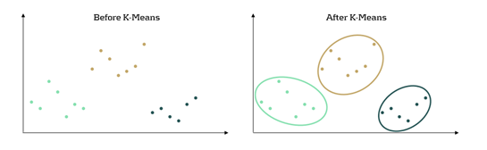
Figure 2: K-Means concept in a 2-dimensional space. Before, the dataset is seen as a whole unstructured dataset while K-means reveals three different segments in the data
Another ML technique useful for segmentation is the decision tree. This method involves splitting the dataset based on certain variables in a way that optimizes a predefined objective. A key advantage of tree-based methods is their interpretability: it is easy to see which variables drive the splits and to assess whether those splits make economic sense. Variable importance measures, like Information Gain, help interpret the decision tree by showing how much each split reduces the entropy (uncertainty). Lower entropy means the data is more organized, allowing for clearer and more meaningful segments to be created.
Estimation
Once the segments are defined, the final step involves applying prediction models to each segment. While the segments resulting from ML models can be used in traditional estimation models such as a logistic regression or a survival model, ML-based estimation models can also be used. An example of such an ML estimation technique is XGBoost. The method combines multiple small decision trees, learning from previous errors, and continuously improving its predictions. It was observed that applying this estimation method in combination with ML-based segments outperformed traditional methods on the used dataset.
Interpretability
Though the techniques show added value, a significant drawback of using ML models for both segmentation and estimation is their tendency to be perceived as black-boxes. A lack of transparency can be problematic for financial institutions, where interpretability is crucial to ensure compliance with regulatory and internal requirements. The SHapley Additive exPlanations (SHAP) method provides an insightful way for explaining predictions made by ML models. The method provides an understanding of a prediction model by showing the average contribution of features across many predictions. SHAP values highlight which features are most important for the model and how they affect the model outcome. This makes it a powerful tool for explaining complex models, by enhancing interpretability and enabling practical use in regulated industries and decision-making processes.
Figure 3 presents an illustrative SHAP plot, showing how different features (variables) influence the ML model’s prepayment rate predictions on a per-observation basis. These features are given on the y-axis, in this case 8 features. Each dot represents a prepayment observation, with its position on the x-axis indicating the SHAP value. This value indicates the impact of that feature on the predicted prepayment rate. Positive values on the x-axis indicate that the feature increased the prediction, while negative values show a decreasing effect. For example, the feature on the bottom indicates that high feature values have a positive effect on the prepayment prediction. This type of plot helps identify the key drivers of prepayment estimates within the model as it can be seen that the bottom two features have the smallest impact on the model output. It also supports stakeholder communication of model results, offering an additional layer of evaluation beyond the conventional in-sample and out-of-sample performance metrics.
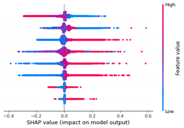
Figure 3: Illustrative SHAP plot
Conclusion
ML techniques can improve prepayment modeling throughout various stages of the model development process, specifically in data processing, segmentation and estimation. By enabling the full potential of ML in these facets, future cashflows can be estimated more precisely, resulting in a more accurate hedge. However, the trade-off between interpretability and accuracy remains an important consideration. Traditional methods offer high transparency and ease of implementation, which is particularly valuable in a heavily regulated financial sector whereas ML models can be considered a black-box. The introduction of explainability techniques such as SHAP help bridge this gap, providing financial institutions with insights into ML model decisions and ensuring compliance with internal and regulatory expectations for model transparency.
In the coming years, (Gen)AI and ML are expected to continue expanding their presence across the financial industry. This creates a growing need to explore opportunities for enhancing model performance, interpretability, and decision-making using these technologies. Beyond prepayment modeling, (Gen)AI and ML techniques are increasingly being applied in areas such as credit risk modeling, fraud detection, stress testing, and treasury analytics.
Zanders has extensive experience in applying advanced analytics across a wide range of financial domains, e.g.:
- Development of a standardized GenAI validation policy for foundational models (i.e., large, general-purpose AI models), ensuring responsible, explainable, and compliant use of GenAI technologies across the organization.
- Application of ML to distinguish between stable and non-stable portions of deposit balances, supporting improved behavioural assumptions for liquidity and interest rate risk management.
- Use of ML in credit risk to monitor the performance and stability of the production Probability of Default (PD) model, enabling early detection of model drift or degradation.
- Deployment of ML to enhance the efficiency and effectiveness of Financial Crime Prevention, including anomaly detection, transaction monitoring, and prioritization of investigative efforts.
Please contact Erik Vijlbrief or Siska van Hees for more information.
Citations
- See Surviving Prepayments: A Comparative Look at Prepayment Modeling Techniques - Zanders for a comparison between both types of models. ↩︎

We investigate different model options for prepayments, among which survival analysis
In brief
- Prepayment modeling can help institutions successfully prepare for and navigate a rise in prepayments due to changes in the financial landscape.
- Two important prepayment modeling types are highlighted and compared: logistic regression vs Cox Proportional Hazard.
- Although the Cox Proportional Hazard model is theoretically preferred under specific conditions, the logical regression is preferred in practice under many scenarios.
The borrowers' option to prepay on their loan induces uncertainty for lenders. How can lenders protect themselves against this uncertainty? Various prepayment modeling approaches can be selected, with option risk and survival analyses being the main alternatives under discussion.
Prepayment options in financial products spell danger for institutions. They inject uncertainty into mortgage portfolios and threaten fixed-rate products with volatile cashflows. To safeguard against losses and stabilize income, institutions must master precise prepayment modeling.
This article delves into the nuances and options regarding the modeling of mortgage prepayments (a cornerstone of Asset Liability Management (ALM)) with a specific focus on survival models.
Understanding the influences on prepayment dynamics
Prepayments are triggered by a range of factors – everything from refinancing opportunities to life changes, such as selling a house due to divorce or moving. These motivations can be grouped into three overarching categories: refinancing factors, macroeconomic factors, and loan-specific factors.
- Refinancing factors
This encompasses key financial drivers (such as interest rates, mortgage rates and penalties) and loan-specific information (including interest rate reset dates and the interest rate differential for the customer). Additionally, the historical momentum of rates and the steepness of the yield curve play crucial roles in shaping refinancing motivations. - Macro-economic factors
The overall state of the economy and the conditions of the housing market are pivotal forces on a borrower's inclination to exercise prepayment options. Furthermore, seasonality adds another layer of variability, with prepayments being notably higher in certain months. For example, in December, when clients have additional funds due to payment of year-end bonusses and holiday budgets. - Loan-specific factors
The age of the mortgage, type of mortgage, and the nature of the property all contribute to prepayment behavior. The seasoning effect, where the probability of prepayment increases with the age of the mortgage, stands out as a paramount factor.
These factors intricately weave together, shaping the landscape in which customers make decisions regarding prepayments. Prepayment modeling plays a vital role in helping institutions to predict the impact of these factors on prepayment behavior.
The evolution of prepayment modeling
Research on prepayment modeling originated in the 1980s and initially centered around option-theoretic models that assume rational customer behavior. Over time, empirical models that cater for customer irrationality have emerged and gained prominence. These models aim to capture the more nuanced behavior of customers by explaining the relationship between prepayment rates and various other factors. In this article, we highlight two important types of prepayment models: logistic regression and Cox Proportional Hazard (Survival Model).
Logistic regression
Logistic regression, specifically its logit or probit variant, is widely employed in prepayment analysis. This is largely because it caters for the binary nature of the dependent variable indicating the occurrence of prepayment events and it moreover flexible. That is, the model can incorporate mortgage-specific and overall economic factors as regressors and can handle time-varying factors and a mix of continuous and categorical variables.
Once the logistic regression model is fitted to historical data, its application involves inputting the characteristics of a new mortgage and relevant economic factors. The model’s output provides the probability of the mortgage undergoing prepayment. This approach is already prevalent in banking practices, and frequently employed in areas such as default modeling and credit scoring. Consequently, it’s favored by many practitioners for prepayment modeling.
Despite its widespread use, the model has drawbacks. While its familiarity in banking scenarios offers simplicity in implementation, it lacks the interpretability characteristic of the Proportional Hazard model discussed below. Furthermore, in terms of robustness, a minimal drawback is that any month-on-month change in results can be caused by numerous factors, which all affect each other.
Cox Proportional Hazard (Survival model)
The Cox Proportional Hazard (PH) model, developed by Sir David Cox in 1972, is one of the most popular models in survival analysis. It consists of two core parts:
- Survival time. With the Cox PH model, the variable of interest is the time to event. As the model stems from medical sciences, this event is typically defined as death. The time variable is referred to as survival time because it’s the time a subject has survived over some follow-up period.
- Hazard rate. This is the distribution of the survival time and is used to predict the probability of the event occurring in the next small-time interval, given that the event has not occurred beforehand. This hazard rate is modelled based on the baseline hazard (the time development of the hazard rate of an average patient) and a multiplier (the effect of patient-specific variables, such as age and gender). An important property of the model is that the baseline hazard is an unspecified function.
To explain how this works in the context of prepayment modeling for mortgages:
- The event of interest is the prepayment of a mortgage.
- The hazard rate is the probability of a prepayment occurring in the next month, given that the mortgage has not been prepaid beforehand. Since the model estimates hazard rates of individual mortgages, it’s modelled using loan-level data.
- The baseline hazard is the typical prepayment behavior of a mortgage over time and captures the seasoning effect of the mortgage.
- The multiplier of the hazard rate is based on mortgage-specific variables, such as the interest rate differential and seasonality.
For full prepayments, where the mortgage is terminated after the event, the Cox PH model applies in its primary format. However, partial prepayments (where the event is recurring) require an extended version, known as the recurrent event PH model. As a result, when using the Cox PH model, , the modeling of partial and full prepayments should be conducted separately, using slightly different models.
The attractiveness of the Cox PH model is due to several features:
- The interpretability of the model. The model makes it possible to quantify the influence of various factors on the likelihood of prepayment in an intuitive way.
- The flexibility of the model. The model offers the flexibility to handle time-varying factors and a mix of continuous and categorical variables, as well as the ability to incorporate recurrent events.
- The multiplier means the hazard rate can’t be negative. The exponential nature of mortgage-specific variables ensures non-negative estimated hazard rates.
Despite the advantages listed above presenting a compelling theoretical case for using the Cox PH model, it faces limited adoption in practical prepayment modeling by banks. This is primarily due to its perceived complexity and unfamiliarity. In addition, when loan-level data is unavailable, the Cox PH model is no longer an option for prepayment modeling.
Logistic regression vs Cox Proportional Hazard
In scenarios with individual survival time data and censored observations, the Cox PH model is theoretically preferred over logistic regression. This preference arises because the Cox PH model leverages this additional information, whereas logistic regression focuses solely on binary outcomes, disregarding survival time and censoring.
However, practical considerations also come into play. Research shows that in certain cases, the logistic regression model closely approximates the results of the Cox PH model, particularly when hazard rates are low. Given that prepayments in the Netherlands are around 3-10% and associated hazard rates tend to be low, the performance gap between logistic regression and the Cox PH model is minimal in practice for this application. Also, the necessity to create a different PH model for full and partial prepayment adds an additional burden on ALM teams.
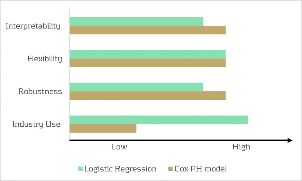
In conclusion, when faced with the absence of loan-level data, the logistic regression model emerges as a pragmatic choice for prepayment modeling. Despite the theoretical preference for the Cox PH model under specific conditions, the real-world performance similarities, coupled with the familiarity and simplicity of logistic regression, provide a practical advantage in many scenarios.
How can Zanders support?
Zanders is a thought leader on IRRBB-related topics. We enable banks to achieve both regulatory compliance and strategic risk goals by offering support from strategy to implementation. This includes risk identification, formulating a risk strategy, setting up an IRRBB governance and framework, and policy or risk appetite statements. Moreover, we have an extensive track record in IRRBB and behavioral models such as prepayment models, hedging strategies, and calculating risk metrics, both from model development and model validation perspectives.
Are you interested in IRRBB-related topics such as prepayments? Contact Jaap Karelse, Erik Vijlbrief, Petra van Meel (Netherlands, Belgium and Nordic countries) or Martijn Wycisk (DACH region) for more information.

At Zanders we have developed several Credit Rating models. These models are already being used at over 400 companies and have been tested both in practice and against empirical data. Do you want to know more about our Credit Rating models, keep reading.
During the development of these models an important step is the calibration of the parameters to ensure a good model performance. In order to maintain these models a regular re-calibration is performed. For our Credit Rating models we strive to rely on a quantitative calibration approach that is combined and strengthened with expert option. This article explains the calibration process for one of our Credit Risk models, the Corporate Rating Model.
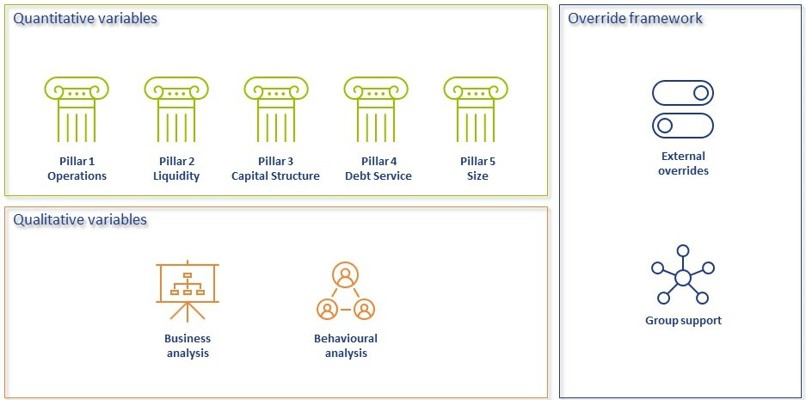
In short, the Corporate Rating Model assigns a credit rating to a company based on its performance on quantitative and qualitative variables. The quantitative part consists of 5 financial pillars; Operations, Liquidity, Capital Structure, Debt Service and Size. The qualitative part consist of 2 pillars; Business Analysis pillar and Behavioural Analysis pillar. See A comprehensive guide to Credit Rating Modeling for more details on the methodology behind this model.
The model calibration process for the Corporate Rating Model can be summarized as follows:
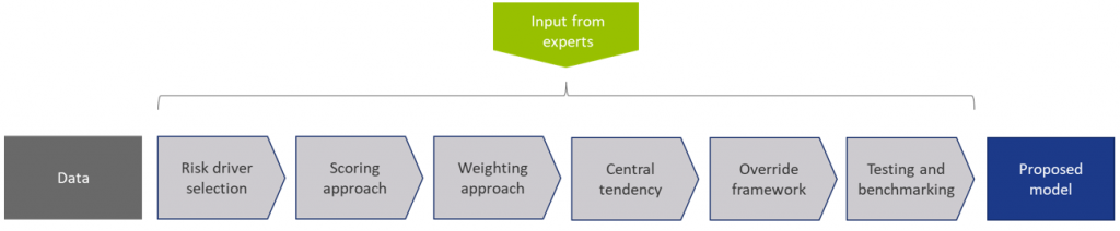
Figure 1: Overview of the model calibration process
In steps (2) through (7), input from the Zanders expert group is taken into consideration. This especially holds for input parameters that cannot be directly derived by a quantitative analysis. For these parameters, first an expert-based baseline value is determined and second a model performance optimization is performed to set the final model parameters.
In most steps the model performance is accessed by looking at the AUC (area under the ROC curve). The AUC metric is one of the most popular metrics to quantify the model fit (note this is not necessarily the same as the model quality, just as correlation does not equal causation). The AUC metric indicates, very simply put, the number of correct and incorrect predictions and plots them in a graph. The area under that graph then indicates the explanatory power of the model
DATA
The first step covers the selection of data from an extensive database containing the financial information and default history of millions of companies. Not all data points can be used in the calibration and/or during the performance testing of the model, therefore data filters are applied. Furthermore, the data set is categorized in 3 different size classes and 18 different industry sectors, each of which will be calibrated independently, using the same methodology.
This results in the master dataset, in addition data statistics are created that show the data availability, data relations and data quality. The master dataset also contains derived fields based on financials from the database, these fields are based on a long list of quantitative risk drivers (financial ratios). The long list of risk drivers is created based on expert option. As a last step, the master dataset is split into a calibration dataset (2/3 of the master dataset) and a test dataset (1/3 of the master dataset).
RISK DRIVER SELECTION
The risk driver selection for the qualitative variables is different from the risk driver selection for the quantitative variables. The final list of quantitative risk drivers is selected by means of different statistical analyses calculated for the long list of quantitative risk drivers. For the qualitative variables, a set of variables is selected based on expert opinion and industry practices.
SCORING APPROACH
Scoring functions are calibrated for the quantitative part of the model. These scoring function translate the value and trend value of each quantitative risk driver per size and industry to a (uniform) score between 0-100. For this exercise, different possible types of scoring functions are used. The best-performing scoring function for the value and trend of each risk driver is determined by performing a regression and comparing the performance. The coefficients in the scoring functions are estimated by fitting the function to the ratio values for companies in the calibration dataset. For the qualitative variables the translation from a value to a score is based on expert opinion.
WEIGHTING APPROACH
The overall score of the quantitative part of the model is combined by summing the value and trend scores by applying weights. As a starting point expert opinion-based weights are applied, after which the performance of the model is further optimized by iteratively adjusting the weights and arriving at an optimal set of weights. The weights of the qualitative variables are based on expert opinion.
MAPPING TO CENTRAL TENDENCY
To estimate the mapping from final scores to a rating class, a standardized methodology is created. The buckets are constructed from a scoring distribution perspective. This is done to ensure the eventual smooth distribution over the rating classes. As an input, the final scores (based on the quantitative risk drivers only) of each company in the calibration dataset is used together with expert opinion input parameters. The estimation is performed per size class. An optimization is performed towards a central tendency by adjusting the expert opinion input parameters. This is done by deriving a target average PD range per size class and on total level based on default data from the European Banking Authority (EBA).
The qualitative variables are included by performing an external benchmark on a selected set of companies, where proxies are used to derive the score on the qualitative variables.
The final input parameters for the mapping are set such that the average PD per size class from the Corporate Rating Model is in line with the target average PD ranges. And, a good performance on the external benchmark is achieved.
OVERRIDE FRAMEWORK
The override framework consists of two sections, Level A and Level B. Level A takes country, industry and company-specific risks into account. Level B considers the possibility of guarantor support and other (final) overriding factors. By applying Level A overrides, the Interim Credit Risk Rating (CRR) is obtained. By applying Level B overrides, the Final CRR is obtained. For the calibration only the country risk is taken into account, as this is the only override that is based on data and not a user input. The country risk is set based on OECD country risk classifications.
TESTING AND BENCHMARKING
For the testing and benchmarking the performance of the model is analysed based on the calibration and test dataset (excluding the qualitative assessment but including the country risk adjustment). For each dataset the discriminatory power is determined by looking at the AUC. The calibration quality is reviewed by performing a Binomial Test on Individual Rating Classes to check if the observed default rate lies within the boundaries of the PD rating class and a Traffic Lights Approach to compare the observed default rates with the PD of the rating class.
Concluding, the methodology applied for the (re-)calibration of the Corporate Rating Model is based on an extensive dataset with financial and default information and complemented with expert opinion. The methodology ensures that the final model performs in-line with the central tendency and an performs well on an external benchmark.

For banks, using variable savings as a source of financing differs fundamentally from ‘professional’ sources of financing.
For banks, using variable savings as a source of financing differs fundamentally from ‘professional’ sources of financing. What risks are involved and how do you determine the return? With capital market financing, such as bond financing, the redemption is known in advance and the interest coupon is fixed for a longer period of time. Financing using variable savings differs from this on two points: the client can withdraw the money at any given time and the bank has the right to adjust the interest rate when it wants to. An essential question here is: why would a bank opt to use savings for financing rather than other sources of financing? The answer to this question is not a simple one, but has to do with the relationship between risk and return.
DETERMINING RETURNS ON THE SAVINGS PORTFOLIO
How do you determine the yield on savings? In order to get as accurate an estimate as possible of the return on a balance sheet instrument, the client rate for a product is often compared to what is called the internal benchmark price, also referred to as the ‘funds transfer price’ (FTP). For savings, the FTP represents the theoretical yield achieved from investing these funds. The difference between the theoretical yield and the actual costs (which includes not only the costs of paying interest on savings, but also the operating/IT costs, for instance) can be regarded as the return on the savings. Calculating this theoretical yield is not a simple task, however. It is often based on a notional investment portfolio, with the same interest rate and liquidity periods as the savings. These periods reflect the interest rate and liquidity characteristics of the savings.
"By ensuring that the expected outflow of savings coincides with the expected influx from investments, the liquidity requirements can be satisfied in the future as well."
MANAGING MARGIN RISK
The question that now arises is: what risks do the savings pose for the bank? Fluctuating market interest rates have an impact on both the yields on the investments and the interest costs on the savings. Although the bank has the right to set its own interest rate, there is a great deal of dependency since banks often follow the interest rate of the market (i.e., their competitors) in order to retain their volume of savings. The bank is therefore exposed to margin risk if the income from the investments does not keep pace with the savings rate offered to clients.
The risk-free interest rate is often the biggest driver behind these kinds of movements on the market for savings interest. The dependency between the savings interest and risk-free interest is indicated using the (estimated) interest rate period. This information makes it possible to mitigate the margin risk in two ways. The interest rate period of the investment portfolio can be aligned with the savings, which causes this income to respond to the interest-free interest rate to the same degree as the costs of paying the savings interest rate. It is also possible to enter into interest rate swaps to influence the interest rate period of the investments.
ASSESSING LIQUIDITY RISK
The liquidity risk of savings manifests if clients withdraw their money and the bank does not have enough cash/liquid investments to comply with these withdrawals. By ensuring that the expected outflow of savings coincides with the expected influx from investments, the liquidity requirements can be satisfied in the future as well. Consequently a bank will be less likely to find itself forced to raise financing or sell illiquid investments in crisis situations. A bank also maintains liquidity buffers for its liquidity requirements in the short term; the regulator requires it to do this by means of the LCR (Liquidity Coverage Ratio) requirement. Since it is expensive to maintain liquidity buffers, a bank aims for a prudent liquidity buffer, but one that is as low as possible. It is also essential for the bank to determine the liquidity period (how long savings remain in the client’s account). It must do this in order to manage the liquidity risk, but also to determine the right level of cash buffers, which improves the return. Savings modeling is a must In order to get the right insight into savings - and to manage them - it is essential to determine both the interest rate period and liquidity period of those savings. It is only with this information that management can gain insight into how the return on savings relates to the margin and liquidity risk.
Regulators are also putting increasing pressure on banks to have better insight into savings. In interest rate risk management, for instance, DNB requires that the interest rate risk of savings be properly substantiated. There is also increasing attention to this from the standpoint of liquidity risk management, for instance as part of the ILAAP (Internal Liquidity Adequacy Assessment Process). Modeling of savings is therefore an absolute must for banks.
GROWING INTEREST IN SAVINGS
At the end of 2012, approximately EUR 950 million of the total of EUR 2.7 billion on Dutch banks’ balance sheets was financed with private savings. EUR 545 million of this comes from Dutch households and businesses. Given the fact that the credit extended to this sector totals EUR 997 million, the Dutch funding gap is the highest of all the euro-zone countries except for Ireland. Since the start of the financial crisis in 2008, there have been two developments that have contributed to the growing interest in savings on the part of banks. First of all, after the collapse of the (inter-bank) money and capital markets, banks had to seek out alternative stable sources of financing. Secondly, compared to other forms of financing, savings have secured a relatively favourable position in the liquidity regulations under Basel III. This culminated in a price war on the savings market in 2010.

Credit rating agencies and the credit ratings they publish have been the subject of a lot of debate over the years. While they provide valuable insight in the creditworthiness of companies, they have been criticized for assigning high ratings to package sub-prime mortgages, for not being representative when a sudden crisis hits and the effect they have on creating ‘self fulfilling prophecies’ in times of economic downturn.
For all the criticism that rating models and credit rating agencies have had through the years, they are still the most pragmatic and realistic approach for assessing default risk for your counterparties. Of course, the quality of the assessment depends to a large extent on the quality of the model used to determine the credit rating, capturing both the quantitative and qualitative factors determining counterparty credit risk. A sound credit rating model strikes a balance between these two aspects. Relying too much on quantitative outcomes ignores valuable ‘unstructured’ information, whereas an expert judgement based approach ignores the value of empirical data, and their explanatory power.
In this white paper we will outline some best practice approaches to assessing default risk of a company through a credit rating. We will explore the ratios that are crucial factors in the model and provide guidance for the expert judgement aspects of the model.
Zanders has applied these best practices while designing several Credit Rating models for many years. These models are already being used at over 400 companies and have been tested both in practice and against empirical data. Do you want to know more about our Credit Rating models, click here.
Credit ratings and their applications
Credit ratings are widely used throughout the financial industry, for a variety of applications. This includes the corporate finance, risk and treasury domains and beyond. While it is hardly ever a sole factor driving management decisions, the availability of a point estimation to describe something as complex as counterparty credit risk has proven a very useful piece of information for making informed decisions, without the need for a full due diligence into the books of the counterparty.
Some of the specific use cases are:
- Internal assessment of the creditworthiness of counterparties
- Transparency of the creditworthiness of counterparties
- Monitoring trends in the quality of credit portfolios
- Monitoring concentration risk
- Performance measurement
- Determination of risk-adjusted credit approval levels and frequency of credit reviews
- Formulation of credit policies, risk appetite, collateral policies, etc.
- Loan pricing based on Risk Adjusted Return on Capital (RAROC) and Economic Profit (EP)
- Arm’s length pricing of intercompany transactions, in line with OECD guidelines
- Regulatory Capital (RC) and Economic Capital (EC) calculations
- Expected Credit Loss (ECL) IFRS 9 calculations
- Active Credit Portfolio Management on both portfolio and (individual) counterparty level
Credit rating philosophy
A fundamental starting point when applying credit ratings, is the credit rating philosophy that is followed. In general, two distinct approaches are recognized:
- Through-the-Cycle (TtC) rating systems measure default risk of a counterparty by taking permanent factors, like a full economic cycle, into account based on a worst-case scenario. TtC ratings change only if there is a fundamental change in the counterparty’s situation and outlook. The models employed for the public ratings published by e.g. S&P, Fitch and Moody’s are generally more TtC focused. They tend to assign more weight to qualitative features and incorporate longer trends in the financial ratios, both of which increase stability over time.
- Point-in-Time (PiT) rating systems measure default risk of a counterparty taking current, temporary factors into account. PiT ratings tend to adjust quickly to changes in the (financial) conditions of a counterparty and/or its economic environment. PiT models are more suited for shorter term risk assessments, like Expected Credit Losses. They are more focused on financial ratios, thereby capturing the more dynamic variables. Furthermore, they incorporate a shorter trend which adjusts faster over time. Most models incorporate a blend between the two approaches, acknowledging that both short term and long term effects may impact creditworthiness.
Rating methodology
Modeling credit ratings is very complex, due to the wide variety of events and exposures that companies are exposed to. Operational risk, liquidity risk, poor management, a perishing business model, an external negative event, failing governments and technological innovation can all have very significant influence on the creditworthiness of companies in the short and long run. Most credit rating models therefore distinguish a range of different factors that are modelled separately and then combined into a single credit rating. The exact factors will differ per rating model. The overview below presents the factors included the Corporate Rating Model, which is used in some of the cloud-based solutions of the Zanders applications.
The remainder of this article will detail the different factors, explaining the rationale behind including them.
Quantitative factors
Quantitative risk factors are crucial to credit rating models, as they are ‘objective’ and therefore generate a large degree of comparability between different companies. Their objective nature also makes them easier to incorporate in a model on a large scale. While financials alone do not tell the whole story about a company, accounting standards have developed over time to provide a more and more comparable view of the financial state of a company, making them a more and more thrustworthy source for determining creditworthiness. To better enable comparisons of companies with different sizes, financials are often represented as ratios.
Financial Ratios
Financial ratios are being used for credit risk analyses throughout the financial industry and present the basic characteristics of companies. A number of these ratios represent (directly or indirectly) creditworthiness. Zanders’ Corporate Credit Rating model uses the most common of these financial ratios, which can be categorised in five pillars:
Pillar 1 - Operations
The Operations pillar consists of variables that consider the profitability and ability of a company to influence its profitability. Earnings power is a main determinant of the success or failure of a company. It measures the ability of a company to create economic value and the ability to give risk protection to its creditors. Recurrent profitability is a main line of defense against debtor-, market-, operational- and business risk losses.
Turnover Growth
Turnover growth is defined as the annual percentage change in Turnover, expressed as a percentage. It indicates the growth rate of a company. Both very low and very high values tend to indicate low credit quality. For low turnover growth this is clear. High turnover growth can be an indication for a risky business strategy or a start-up company with a business model that has not been tested over time.
Gross Margin
Gross margin is defined as Gross profit divided by Turnover, expressed as a percentage. The gross margin indicates the profitability of a company. It measures how much a company earns, taking into consideration the costs that it incurs for producing its products and/or services. A higher Gross margin implies a lower default probability.
Operating Margin
Operating margin is defined as Earnings before Interest and Taxes (EBIT) divided by Turnover, expressed as a percentage. This ratio indicates the profitability of the company. Operating margin is a measurement of what proportion of a company's revenue is left over after paying for variable costs of production such as wages, raw materials, etc. A healthy Operating margin is required for a company to be able to pay for its fixed costs, such as interest on debt. A higher Operating margin implies a lower default probability.
Return on Sales
Return on sales is defined as P/L for period (Net income) divided by Turnover, expressed as a percentage. Return on sales = P/L for period (Net income) / Turnover x 100%. Return on sales indicates how much profit, net of all expenses, is being produced per pound of sales. Return on sales is also known as net profit margin. A higher Return on sales implies a lower default probability.
Return on Capital Employed
Return on capital employed (ROCE) is defined as Earnings before Interest and Taxes (EBIT) divided by Total assets minus Current liabilities, expressed as a percentage. This ratio indicates how successful management has been in generating profits (before Financing costs) with all of the cash resources provided to them which carry a cost, i.e. equity plus debt. It is a basic measure of the overall performance, combining margins and efficiency in asset utilization. A higher ROCE implies a lower default probability.
Pillar 2 - Liquidity
The Liquidity pillar assesses the ability of a company to become liquid in the short-term. Illiquidity is almost always a direct cause of a failure, while a strong liquidity helps a company to remain sufficiently funded in times of distress. The liquidity pillar consists of variables that consider the ability of a company to convert an asset into cash quickly and without any price discount to meet its obligations.
Current Ratio
Current ratio is defined as Current assets, including Cash and Cash equivalents, divided by Current liabilities, expressed as a number. This ratio is a rough indication of a firm's ability to service its current obligations. Generally, the higher the Current ratio, the greater the cushion between current obligations and a firm's ability to pay them. A stronger ratio reflects a numerical superiority of Current assets over Current liabilities. However, the composition and quality of Current assets are a critical factor in the analysis of an individual firm's liquidity, which is why the current ratio assessment should be considered in conjunction with the overall liquidity assessment. A higher Current ratio implies a lower default probability.
Quick Ratio
The Quick ratio (also known as the Acid test ratio) is defined as Current assets, including Cash and Cash equivalents, minus Stock divided by Current liabilities, expressed as a number. The ratio indicates the degree to which a company's Current liabilities are covered by the most liquid Current assets. It is a refinement of the Current ratio and is a more conservative measure of liquidity. Generally, any value of less than 1 to 1 implies a reciprocal dependency on inventory or other current assets to liquidate short-term debt. A higher Quick ratio implies a lower default probability.
Stock Days
Stock days is defined as the average Stock during the year times the number of days in a year divided by the Cost of goods sold, expressed as a number. This ratio indicates the average length of time that units are in stock. A low ratio is a sign of good liquidity or superior merchandising. A high ratio can be a sign of poor liquidity, possible overstocking, obsolescence, or, in contrast to these negative interpretations, a planned stock build-up in the case of material shortages. A higher Stock days ratio implies a higher default probability.
Debtor Days
Debtor days is defined as the average Debtors during the year times the number of days in a year divided by Turnover. Debtor days indicates the average number of days that trade debtors are outstanding. Generally, the greater number of days outstanding, the greater the probability of delinquencies in trade debtors and the more cash resources are absorbed. If a company's debtors appear to be turning slower than the industry, further research is needed and the quality of the debtors should be examined closely. A higher Debtors days ratio implies a higher default probability.
Creditor Days
Creditor days is defined as the average Creditors during the year as a fraction of the Cost of goods sold times the number of days in a year. It indicates the average length of time the company's trade debt is outstanding. If a company's Creditors days appear to be turning more slowly than the industry, then the company may be experiencing cash shortages, disputing invoices with suppliers, enjoying extended terms, or deliberately expanding its trade credit. The ratio comparison of company to industry suggests the existence of these or other causes. A higher Creditors days ratio implies a higher default probability.
Pillar 3 - Capital Structure
The Capital pillar considers how a company is financed. Capital should be sufficient to cover expected and unexpected losses. Strong capital levels provide management with financial flexibility to take advantage of certain acquisition opportunities or allow discontinuation of business lines with associated write offs.
Gearing
Gearing is defined as Total debt divided by Tangible net worth, expressed as a percentage. It indicates the company’s reliance on (often expensive) interest bearing debt. In smaller companies, it also highlights the owners' stake in the business relative to the banks. A higher Gearing ratio implies a higher default probability.
Solvency
Solvency is defined as Tangible net worth (Shareholder funds – Intangibles) divided by Total assets – Intangibles, expressed as a percentage. It indicates the financial leverage of a company, i.e. it measures how much a company is relying on creditors to fund assets. The lower the ratio, the greater the financial risk. The amount of risk considered acceptable for a company depends on the nature of the business and the skills of its management, the liquidity of the assets and speed of the asset conversion cycle, and the stability of revenues and cash flows. A higher Solvency ratio implies a lower default probability.
Pillar 4 - Debt Service
The debt service pillar considers the capability of a company to meet its financial obligations in the form of debt. It ties the debt obligation a company has to its earnings potential.
Total Debt / EBITDA
The debt service pillar considers the capability of a company to meet its financial obligations. This ratio is defined as Total debt divided by Earnings before Interest, Taxes, Depreciation, and Amortization (EBITDA). Total debt comprises Loans + Noncurrent liabilities. It indicates the total debt run-off period by showing the number of years it would take to repay all of the company's interest-bearing debt from operating profit adjusted for Depreciation and Amortization. However, EBITDA should not, of course, be considered as cash available to pay off debt. A higher Debt service ratio implies a higher default probability.
Interest Coverage Ratio
Interest coverage ratio is defined as Earnings before interest and taxes (EBIT) divided by interest expenses (Gross and Capitalized). It indicates the firm's ability to meet interest payments from earnings. A high ratio indicates that the borrower should have little difficulty in meeting the interest obligations of loans. This ratio also serves as an indicator of a firm's ability to service current debt and its capacity for taking on additional debt. A higher Interest coverage ratio implies a lower default probability.
Pillar 5 - Size
In general, the larger a company is, the less vulnerable the company is, as there is, usually, more diversification in turnover. Turnover is considered the best indicator of size. In general, turnover is related to vulnerability. The higher the turnover, the less vulnerable a company (generally) is.
Ratio Scoring and Mapping
While these financial ratios provide some very useful information regarding the current state of a company, it is difficult to assess them on a stand-alone basis. They are only useful in a credit rating determination if we can compare them to the same ratios for a group of peers. Ratio scoring deals with the process of translating the financials to a score that gives an indication of the relative creditworthiness of a company against its peers.
The ratios are assessed against a peer group of companies. This provides more discriminatory power during the calibration process and hence a better estimation of the risk that a company will default. Research has shown that there are two factors that are most fundamental when determining a comparable peer group. These two factors are industry type and size. The financial ratios tend to behave ‘most alike’ within these segmentations. The industry type is a good way to separate, for example, companies with a lot of tangible assets on their balance sheet (e.g. retail) versus companies with very few tangible assets (e.g. service based industries). The size reflects that larger companies are generally more robust and less likely to default in the short to medium term, as compared to smaller, less mature companies.
Since ratios tend to behave differently over different industries and sizes, the ratio value score has to be calibrated for each peer group segment.
When scoring a ratio, both the latest value and the long-term trend should be taken into account. The trend reflects whether a company’s financials are improving or deteriorating over time, which may be an indication of their long-term perspective. Hence, trends are also taken into account as a separate factor in the scoring function.
To arrive to a total score, a set of weights needs to be determined, which indicates the relative importance of the different components. This total score is then mapped to a ordinal rating scale, which usually runs from AAA (excellent creditworthiness) to D (defaulted) to indicate the creditworthiness. Note that at this stage, the rating only incorporates the quantitative factors. It will serve as a starting point to include the qualitative factors and the overrides.
"A sound credit rating model strikes a balance between quantitative and qualitative aspects. Relying too much on quantitative outcomes ignores valuable ‘unstructured’ information, whereas an expert judgement based approach ignores the value of empirical data, and their explanatory power."
Qualitative Factors
Qualitative factors are crucial to include in the model. They capture the ‘softer’ criteria underlying creditworthiness. They relate, among others, to the track record, management capabilities, accounting standards and access to capital of a company. These can be hard to capture in concrete criteria, and they will differ between different credit rating models.
Note that due to their qualitative nature, these factors will rely more on expert opinion and industry insights. Furthermore, some of these factors will affect larger companies more than smaller companies and vice versa. In larger companies, management structures are far more complex, track records will tend to be more extensive and access to capital is a more prominent consideration.
All factors are generally assigned an ordinal scoring scale and relative weights, to arrive at a total score for the qualitative part of the assessment.
A categorisation can be made between business analysis and behavioural analysis.
Business Analysis
Business analysis deals with all aspects of a company that relate to the way they operate in the markets. Some of the factors that can be included in a credit rating model are the following:
Years in Same Business
Companies that have operated in the same line of business for a prolonged period of time have increased credibility of staying around for the foreseeable future. Their business model is sound enough to generate stable financials.
Customer Risk
Customer risk is an assessment to what extent a company is dependent on one or a small group of customers for their turnover. A large customer taking its business to a competitor can have a significant impact on such a company.
Accounting Risk
The companies internal accounting standards are generally a good indicator of the quality of management and internal controls. Recent or frequent incidents, delayed annual reports and a lack of detail are clear red flags.
Track record with Corporate
This is mostly relevant for counterparties with whom a standing relationship exists. The track record of previous years is useful first hand experience to take into account when assessing the creditworthiness.
Continuity of Management
A company that has been under the same management for an extended period of time tends to reflect a stable company, with few internal struggles. Furthermore, this reflects a positive assessment of management by the shareholders.
Operating Activities Area
Companies operating on a global scale are generally more diversified and therefore less affected by most political and regulatory risks. This reflects well in their credit rating. Additionally, companies that serve a large market have a solid base that provides some security against adverse events.
Access to Capital
Access to capital is a crucial element of the qualitative assessment. Companies with a good access to the capital markets can raise debt and equity as needed. An actively traded stock, a public rating and frequent and recent debt issuances are all signals that a company has access to capital.
Behavioral Analysis
Behavioural analysis aims to incorporate prior behaviour of a company in the credit rating. A separation can be made between external and internal indicators
External indicators
External indicators are all information that can be acquired from external parties, relating to the behaviour of a company where it comes to honouring obligations. This could be a credit rapport from a credit rating agency, payment details from a bank, public news items, etcetera.
Internal Indicators
Internal indicators concern all prior interactions you have had with a company. This includes payment delay, litigation, breaches of financial covenants etcetera.
Override Framework
Many models allow for an override of the credit rating resulting from the prior analysis. This is a more discretionary step, which should be properly substantiated and documented. Overrides generally only allow for adjusting the credit rating with one notch upward, while downward adjustment can be more sizable.
Overrides can be made due to a variety of reasons, which is generally carefully separated in the model. Reasons for overrides generally include adjusting for country risk, industry adjustments, company specific risk and group support.
It should be noted that some overrides are mandated by governing bodies. As an example, the OECD prescribes the overrides to be applied based on a country risk mapping table, for the purpose of arm’s length pricing of intercompany contracts.
Combining all the factors and considerations mentioned in this article, applying weights and scoring functions and applying overrides, a final credit rating results.
Model Quality and Fit
The model quality determines whether the model is appropriate to be used in a practical setting. From a statistical modeling perspective, a lot of considerations can be made with regard to model quality, which are outside of the scope of this article, so we will stick to a high level consideration here.
The AUC (area under the ROC curve) metric is one of the most popular metrics to quantify the model fit (note this is not necessarily the same as the model quality, just as correlation does not equal causation). The AUC metric indicates, very simply put, the number of correct and incorrect predictions and plots them in a graph. The area under that graph then indicates the explanatory power of the model. A more extensive guide to the AUC metric can be found here.
Alternative Modeling Approaches
The model structure described above is one specific way to model credit ratings. While models may widely vary, most of these components would typically be included. During recent years, there has been an increase in the use of payment data, which is disclosed through the PSD2 regulation. This can provide a more up-to-date overview of the state of the company and can definitely be considered as an additional factor in the analysis. However, the main disadvantage of this approach is that it requires explicit approval from the counterparty to use the data, which makes it more challenging to apply on a portfolio basis.
Another approach is a purely machine learning based modeling approach. If applied well, this will give the best model in terms of the AUC (area under the curve) metric, which measures the explanatory power of the model. One major disadvantage of this approach, however, is that the interpretability of the resulting model is very limited. This is something that is generally not preferred by auditors and regulatory bodies as the primary model for creditworthiness. In practice, we see these models most often as challenger models, to benchmark the explanatory power of models based on economic rationale. They can serve to spot deficiencies in the explanatory power of existing models and trigger a re-assessment of the factors included in these models. In some cases, they may also be used to create additional comfort regarding the inclusion of some factors.
Furthermore, the degree to which the model depends on expert opinion is to a large extent dependent on the data available to the model developer. Most notably, the financials and historical default data of a representative group of companies is needed to properly fit the model to the empirical data. Since this data can be hard to come by, many credit rating models are based more on expert opinion than actual quantitative data. Our Corporate Credit Rating model was calibrated on a database containing the financials and default data of an extensive set of companies. This provides a solid quantitative basis for the model outcomes.
Closing Remarks
Model credit risk and credit ratings is a complex affair. Zanders provides advice, standardized and customizable models and software solutions to tackle these challenges. Do you want to learn more about credit rating modeling? Reach out for a free consultation. Looking for a tailor made and flexible solution to become IFRS 9 compliant, find out about our Condor Credit Risk Suite, the IFRS9 compliance solution.


