INTRODUCTION

The IFRS 9 accounting standard has been effective since 2018 and affects both financial institutions and corporates. Although the IFRS 9 standards are principle-based and simple, the design and implementation can be challenging. Specifically, the difficulties that the incorporation of forward-looking information in the loss estimate introduces should not be underestimated. Using our hands-on experience and over two decades of credit risk expertise of our consultants, Zanders developed the Credit Risk Suite. The Credit Risk Suite is a calculation engine that determines transaction-level IFRS 9 compliant provisions for credit losses. The CRS was designed specifically to overcome the difficulties that our clients face in their IFRS 9 provisioning. In this article, we will elaborate on the methodology of the ECL calculations that take place in the CRS.

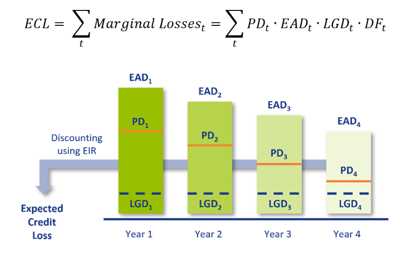
An industry best-practice approach for ECL calculations requires four main ingredients:

• Probability of Default (PD): The probability that a counterparty will default at a certain point in time. This can be a one-year PD, i.e. the probability of defaulting between now and one year, or a lifetime PD, i.e. the probability of defaulting before the maturity of the contract. A lifetime PD can be split into marginal PDs which represent the probability of default in a certain period.
• Exposure at Default (EAD): The exposure remaining until maturity of the contract based on current exposure, contractual, expected redemptions and future drawings on remaining commitments.
• Loss Given Default (LGD): The percentage of EAD that is expected to be lost in case of default. The LGD differs with the level of collateral, guarantees and subordination associated with the financial instrument.
• Discount Factor (DF): The expected loss per period is discounted to present value terms using discount factors. Discount factors according to IFRS 9 are based on the effective interest rate.

The overall ECL calculation is performed as follows and illustrated by the diagram below:

MODEL COMPONENTS

The CRS consists of multiple components and underlying models that are able to calculate each of these ingredients separately. The separate components are then combined into ECL provisions which can be utilized for IFRS 9 accounting purposes. Besides this, the CRS contains a customizable module for scenario-based Forward-Looking Information (FLI). Moreover, the solution allocates assets to one of the three IFRS 9 stages. In the component approach, projections of PDs, EADs and LGDs are constructed separately. This component-based setup of the CRS allows for customizable and easy to implement approach. The methodology that is applied for each of the components is described below.

PROBABILITY OF DEFAULT

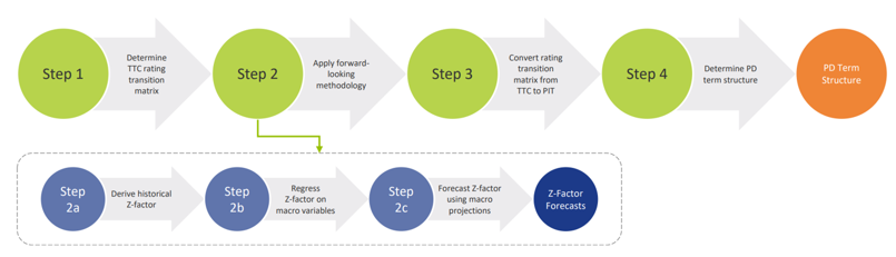
For each projected month, the PD is derived from the PD term structure that is relevant for the portfolio as well as the economic scenario. This is done using the PD module. The purpose of this module is to determine forward-looking Point-in-Time (PIT) PDs for all counterparties. This is done by transforming Through-the-Cycle (TTC) rating migration matrices into PIT rating migration matrices. The TTC rating migration matrices represent the long-term average annual transition PDs, while the PIT rating migration matrices are annual transition PDs adjusted to the current (expected) state of the economy. The PIT PDs are determined in the following steps:

1. Determine TTC rating transition matrices: To be able to calculate PDs for all possible maturities, an approach based on rating transition matrices is applied. A transition matrix specifies the probability to go from a specified rating to another rating in one year time. The TTC rating transition matrices can be constructed using e.g., historical default data provided by the client or external rating agencies.
2. Apply forward-looking methodology: IFRS 9 requires the state of the economy to be reflected in the ECL. In the CRS, the state of the economy is incorporated in the PD by applying a forward-looking methodology. The forward-looking methodology in the CRS is based on a ‘Z-factor approach’, where the Z-factor represents the state of the macroeconomic environment. Essentially, a relationship is determined between historical default rates and specific macroeconomic variables. The approach consists of the following sub-steps:
   1. Derive historical Z-factors from (global or local) historical default rates.
   2. Regress historical Z-factors on (global or local) macro-economic variables.
   3. Obtain Z-factor forecasts using macro-economic projections.
3. Convert rating transition matrices from TTC to PIT: In this step, the forward-looking information is used to convert TTC rating transition matrices to point-in-time (PIT) rating transition matrices. The PIT transition matrices can be used to determine rating transitions in various states of the economy.
4. Determine PD term structure: In the final step of the process, the rating transition matrices are iteratively applied to obtain a PD term structure in a specific scenario. The PD term structure defines the PD for various points in time.

The result of this is a forward-looking PIT PD term structure for all transactions which can be used in the ECL calculations.

EXPOSURE AT DEFAULT

For any given transaction, the EAD consists of the outstanding principal of the transaction plus accrued interest as of the calculation date. For each projected month, the EAD is determined using cash flow data if available. If not available, data from a portfolio snapshot from the reporting date is used to determine the EAD.

LOSS GIVEN DEFAULT

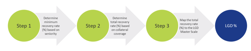
For each projected month, the LGD is determined using the LGD module. This module estimates the LGD for individual credit facilities based on the characteristics of the facility and availability and quality of pledged collateral. The process for determining the LGD consists of the following steps:

1. Seniority of transaction: A minimum recovery rate is determined based on the seniority of the transaction.
2. Collateral coverage: For the part of the loan that is not covered by the minimum recovery rate, the collateral coverage of the facility is determined in order to estimate the total recovery rate.
3. Mapping to LGD class: The total recovery rate is mapped to an LGD class using an LGD scale.

SCENARIO-WEIGHTED AVERAGE EXPECTED CREDIT LOSS

Once all expected losses have been calculated for all scenarios, the weighted average one-year and lifetime loss are calculated for each transaction , for both 1-year and lifetime scenario losses:

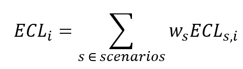
For each scenario , the weights  are predetermined. For each transaction , the scenario losses are weighted according to the formula above, where  is either the lifetime or the one-year expected scenario loss. An example of applied scenarios and corresponding weights is as follows:

• Optimistic scenario: 25%
• Neutral scenario: 50%
• Pessimistic scenario: 25%

This results in a one-year and a lifetime scenario-weighted average ECL estimate for each transaction.

STAGE ALLOCATION

Lastly, using a stage allocation rule, the applicable (i.e., one-year or lifetime) scenario-weighted ECL estimate for each transaction is chosen. The stage allocation logic consists of a customisable quantitative assessment to determine whether an exposure is assigned to Stage 1, 2 or 3. One example could be to use a relative and absolute PD threshold:

• Relative PD threshold: +300% increase in PD (with an absolute minimum of 25 bps)
• Absolute PD threshold: +3%-point increase in PD The PD thresholds will be applied to one-year best estimate PIT PDs.

If either of the criteria are met, Stage 2 is assigned. Otherwise, the transaction is assigned Stage 1.

The provision per transaction are determined using the stage of the transaction. If the transaction stage is Stage 1, the provision is equal to the one-year expected loss. For Stage 2, the provision is equal to the lifetime expected loss. Stage 3 provision calculation methods are often transaction-specific and based on expert judgement.

During the development of these models an important step is the calibration of the parameters to ensure a good model performance. In order to maintain these models a regular re-calibration is performed. For our Credit Rating models we strive to rely on a quantitative calibration approach that is combined and strengthened with expert option. This article explains the calibration process for one of our Credit Risk models, the Corporate Rating Model.

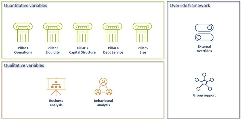
In short, the Corporate Rating Model assigns a credit rating to a company based on its performance on quantitative and qualitative variables. The quantitative part consists of 5 financial pillars; Operations, Liquidity, Capital Structure, Debt Service and Size. The qualitative part consist of 2 pillars; Business Analysis pillar and Behavioural Analysis pillar. See A comprehensive guide to Credit Rating Modelling for more details on the methodology behind this model.

The model calibration process for the Corporate Rating Model can be summarized as follows:

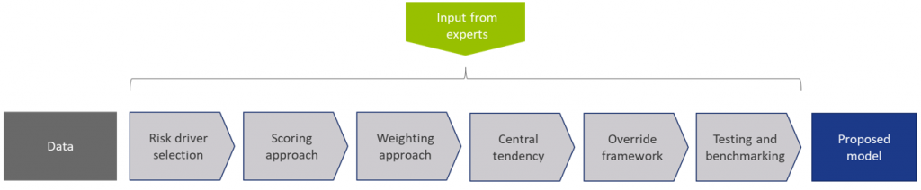
Figure 1: Overview of the model calibration process

In steps (2) through (7), input from the Zanders expert group is taken into consideration. This especially holds for input parameters that cannot be directly derived by a quantitative analysis. For these parameters, first an expert-based baseline value is determined and second a model performance optimization is performed to set the final model parameters.

In most steps the model performance is accessed by looking at the AUC (area under the ROC curve). The AUC metric is one of the most popular metrics to quantify the model fit (note this is not necessarily the same as the model quality, just as correlation does not equal causation). The AUC metric indicates, very simply put, the number of correct and incorrect predictions and plots them in a graph. The area under that graph then indicates the explanatory power of the model

DATA

The first step covers the selection of data from an extensive database containing the financial information and default history of millions of companies. Not all data points can be used in the calibration and/or during the performance testing of the model, therefore data filters are applied. Furthermore, the data set is categorized in 3 different size classes and 18 different industry sectors, each of which will be calibrated independently, using the same methodology.

This results in the master dataset, in addition data statistics are created that show the data availability, data relations and data quality. The master dataset also contains derived fields based on financials from the database, these fields are based on a long list of quantitative risk drivers (financial ratios). The long list of risk drivers is created based on expert option. As a last step, the master dataset is split into a calibration dataset (2/3 of the master dataset) and a test dataset (1/3 of the master dataset).

RISK DRIVER SELECTION

The risk driver selection for the qualitative variables is different from the risk driver selection for the quantitative variables. The final list of quantitative risk drivers is selected by means of different statistical analyses calculated for the long list of quantitative risk drivers. For the qualitative variables, a set of variables is selected based on expert opinion and industry practices.

SCORING APPROACH

Scoring functions are calibrated for the quantitative part of the model. These scoring function translate the value and trend value of each quantitative risk driver per size and industry to a (uniform) score between 0-100. For this exercise, different possible types of scoring functions are used. The best-performing scoring function for the value and trend of each risk driver is determined by performing a regression and comparing the performance. The coefficients in the scoring functions are estimated by fitting the function to the ratio values for companies in the calibration dataset. For the qualitative variables the translation from a value to a score is based on expert opinion.

WEIGHTING APPROACH

The overall score of the quantitative part of the model is combined by summing the value and trend scores by applying weights. As a starting point expert opinion-based weights are applied, after which the performance of the model is further optimized by iteratively adjusting the weights and arriving at an optimal set of weights. The weights of the qualitative variables are based on expert opinion.

MAPPING TO CENTRAL TENDENCY

To estimate the mapping from final scores to a rating class, a standardized methodology is created. The buckets are constructed from a scoring distribution perspective. This is done to ensure the eventual smooth distribution over the rating classes. As an input, the final scores (based on the quantitative risk drivers only) of each company in the calibration dataset is used together with expert opinion input parameters. The estimation is performed per size class. An optimization is performed towards a central tendency by adjusting the expert opinion input parameters. This is done by deriving a target average PD range per size class and on total level based on default data from the European Banking Authority (EBA).

The qualitative variables are included by performing an external benchmark on a selected set of companies, where proxies are used to derive the score on the qualitative variables.

The final input parameters for the mapping are set such that the average PD per size class from the Corporate Rating Model is in line with the target average PD ranges. And, a good performance on the external benchmark is achieved.

OVERRIDE FRAMEWORK

The override framework consists of two sections, Level A and Level B. Level A takes country, industry and company-specific risks into account. Level B considers the possibility of guarantor support and other (final) overriding factors. By applying Level A overrides, the Interim Credit Risk Rating (CRR) is obtained. By applying Level B overrides, the Final CRR is obtained. For the calibration only the country risk is taken into account, as this is the only override that is based on data and not a user input. The country risk is set based on OECD country risk classifications.

TESTING AND BENCHMARKING

For the testing and benchmarking the performance of the model is analysed based on the calibration and test dataset (excluding the qualitative assessment but including the country risk adjustment). For each dataset the discriminatory power is determined by looking at the AUC. The calibration quality is reviewed by performing a Binomial Test on Individual Rating Classes to check if the observed default rate lies within the boundaries of the PD rating class and a Traffic Lights Approach to compare the observed default rates with the PD of the rating class.

Concluding, the methodology applied for the (re-)calibration of the Corporate Rating Model is based on an extensive dataset with financial and default information and complemented with expert opinion. The methodology ensures that the final model performs in-line with the central tendency and an performs well on an external benchmark.

For all the criticism that rating models and credit rating agencies have had through the years, they are still the most pragmatic and realistic approach for assessing default risk for your counterparties. Of course, the quality of the assessment depends to a large extent on the quality of the model used to determine the credit rating, capturing both the quantitative and qualitative factors determining counterparty credit risk. A sound credit rating model strikes a balance between these two aspects. Relying too much on quantitative outcomes ignores valuable ‘unstructured’ information, whereas an expert judgement based approach ignores the value of empirical data, and their explanatory power.

In this white paper we will outline some best practice approaches to assessing default risk of a company through a credit rating. We will explore the ratios that are crucial factors in the model and provide guidance for the expert judgement aspects of the model.

Zanders has applied these best practices while designing several Credit Rating models for many years. These models are already being used at over 400 companies and have been tested both in practice and against empirical data. Do you want to know more about our Credit Rating models, click here.

Credit ratings and their applications

Credit ratings are widely used throughout the financial industry, for a variety of applications. This includes the corporate finance, risk and treasury domains and beyond. While it is hardly ever a sole factor driving management decisions, the availability of a point estimation to describe something as complex as counterparty credit risk has proven a very useful piece of information for making informed decisions, without the need for a full due diligence into the books of the counterparty.

Some of the specific use cases are:

• Internal assessment of the creditworthiness of counterparties
• Transparency of the creditworthiness of counterparties
• Monitoring trends in the quality of credit portfolios
• Monitoring concentration risk
• Performance measurement
• Determination of risk-adjusted credit approval levels and frequency of credit reviews
• Formulation of credit policies, risk appetite, collateral policies, etc.
• Loan pricing based on Risk Adjusted Return on Capital (RAROC) and Economic Profit (EP)
• Arm’s length pricing of intercompany transactions, in line with OECD guidelines
• Regulatory Capital (RC) and Economic Capital (EC) calculations
• Expected Credit Loss (ECL) IFRS 9 calculations
• Active Credit Portfolio Management on both portfolio and (individual) counterparty level

Credit rating philosophy

A fundamental starting point when applying credit ratings, is the credit rating philosophy that is followed. In general, two distinct approaches are recognized:

• Through-the-Cycle (TtC) rating systems measure default risk of a counterparty by taking permanent factors, like a full economic cycle, into account based on a worst-case scenario. TtC ratings change only if there is a fundamental change in the counterparty’s situation and outlook. The models employed for the public ratings published by e.g. S&P, Fitch and Moody’s are generally more TtC focused. They tend to assign more weight to qualitative features and incorporate longer trends in the financial ratios, both of which increase stability over time.
• Point-in-Time (PiT) rating systems measure default risk of a counterparty taking current, temporary factors into account. PiT ratings tend to adjust quickly to changes in the (financial) conditions of a counterparty and/or its economic environment. PiT models are more suited for shorter term risk assessments, like Expected Credit Losses. They are more focused on financial ratios, thereby capturing the more dynamic variables. Furthermore, they incorporate a shorter trend which adjusts faster over time. Most models incorporate a blend between the two approaches, acknowledging that both short term and long term effects may impact creditworthiness.

Rating methodology

Modelling credit ratings is very complex, due to the wide variety of events and exposures that companies are exposed to. Operational risk, liquidity risk, poor management, a perishing business model, an external negative event, failing governments and technological innovation can all have very significant influence on the creditworthiness of companies in the short and long run. Most credit rating models therefore distinguish a range of different factors that are modelled separately and then combined into a single credit rating. The exact factors will differ per rating model. The overview below presents the factors included the Corporate Rating Model, which is used in some of the cloud-based solutions of the Zanders applications.

The remainder of this article will detail the different factors, explaining the rationale behind including them.

Quantitative factors

Quantitative risk factors are crucial to credit rating models, as they are ‘objective’ and therefore generate a large degree of comparability between different companies. Their objective nature also makes them easier to incorporate in a model on a large scale. While financials alone do not tell the whole story about a company, accounting standards have developed over time to provide a more and more comparable view of the financial state of a company, making them a more and more thrustworthy source for determining creditworthiness. To better enable comparisons of companies with different sizes, financials are often represented as ratios.

Financial Ratios

Financial ratios are being used for credit risk analyses throughout the financial industry and present the basic characteristics of companies. A number of these ratios represent (directly or indirectly) creditworthiness. Zanders’ Corporate Credit Rating model uses the most common of these financial ratios, which can be categorised in five pillars:

Pillar 1 - Operations

The Operations pillar consists of variables that consider the profitability and ability of a company to influence its profitability. Earnings power is a main determinant of the success or failure of a company. It measures the ability of a company to create economic value and the ability to give risk protection to its creditors. Recurrent profitability is a main line of defense against debtor-, market-, operational- and business risk losses. 

Turnover Growth

Turnover growth is defined as the annual percentage change in Turnover, expressed as a percentage. It indicates the growth rate of a company. Both very low and very high values tend to indicate low credit quality. For low turnover growth this is clear. High turnover growth can be an indication for a risky business strategy or a start-up company with a business model that has not been tested over time.

Gross Margin

Gross margin is defined as Gross profit divided by Turnover, expressed as a percentage. The gross margin indicates the profitability of a company. It measures how much a company earns, taking into consideration the costs that it incurs for producing its products and/or services. A higher Gross margin implies a lower default probability.

Operating Margin

Operating margin is defined as Earnings before Interest and Taxes (EBIT) divided by Turnover, expressed as a percentage. This ratio indicates the profitability of the company. Operating margin is a measurement of what proportion of a company's revenue is left over after paying for variable costs of production such as wages, raw materials, etc. A healthy Operating margin is required for a company to be able to pay for its fixed costs, such as interest on debt. A higher Operating margin implies a lower default probability.

Return on Sales

Return on sales is defined as P/L for period (Net income) divided by Turnover, expressed as a percentage. Return on sales = P/L for period (Net income) / Turnover x 100%. Return on sales indicates how much profit, net of all expenses, is being produced per pound of sales. Return on sales is also known as net profit margin. A higher Return on sales implies a lower default probability.

Return on Capital Employed

Return on capital employed (ROCE) is defined as Earnings before Interest and Taxes (EBIT) divided by Total assets minus Current liabilities, expressed as a percentage. This ratio indicates how successful management has been in generating profits (before Financing costs) with all of the cash resources provided to them which carry a cost, i.e. equity plus debt. It is a basic measure of the overall performance, combining margins and efficiency in asset utilization. A higher ROCE implies a lower default probability.

Pillar 2 - Liquidity

The Liquidity pillar assesses the ability of a company to become liquid in the short-term. Illiquidity is almost always a direct cause of a failure, while a strong liquidity helps a company to remain sufficiently funded in times of distress. The liquidity pillar consists of variables that consider the ability of a company to convert an asset into cash quickly and without any price discount to meet its obligations. 

Current Ratio

Current ratio is defined as Current assets, including Cash and Cash equivalents, divided by Current liabilities, expressed as a number. This ratio is a rough indication of a firm's ability to service its current obligations. Generally, the higher the Current ratio, the greater the cushion between current obligations and a firm's ability to pay them. A stronger ratio reflects a numerical superiority of Current assets over Current liabilities. However, the composition and quality of Current assets are a critical factor in the analysis of an individual firm's liquidity, which is why the current ratio assessment should be considered in conjunction with the overall liquidity assessment. A higher Current ratio implies a lower default probability. 

Quick Ratio

The Quick ratio (also known as the Acid test ratio) is defined as Current assets, including Cash and Cash equivalents, minus Stock divided by Current liabilities, expressed as a number. The ratio indicates the degree to which a company's Current liabilities are covered by the most liquid Current assets. It is a refinement of the Current ratio and is a more conservative measure of liquidity. Generally, any value of less than 1 to 1 implies a reciprocal dependency on inventory or other current assets to liquidate short-term debt. A higher Quick ratio implies a lower default probability.

Stock Days 

Stock days is defined as the average Stock during the year times the number of days in a year divided by the Cost of goods sold, expressed as a number. This ratio indicates the average length of time that units are in stock. A low ratio is a sign of good liquidity or superior merchandising. A high ratio can be a sign of poor liquidity, possible overstocking, obsolescence, or, in contrast to these negative interpretations, a planned stock build-up in the case of material shortages. A higher Stock days ratio implies a higher default probability.

Debtor Days

Debtor days is defined as the average Debtors during the year times the number of days in a year divided by Turnover. Debtor days indicates the average number of days that trade debtors are outstanding. Generally, the greater number of days outstanding, the greater the probability of delinquencies in trade debtors and the more cash resources are absorbed. If a company's debtors appear to be turning slower than the industry, further research is needed and the quality of the debtors should be examined closely. A higher Debtors days ratio implies a higher default probability.

Creditor Days

Creditor days is defined as the average Creditors during the year as a fraction of the Cost of goods sold times the number of days in a year. It indicates the average length of time the company's trade debt is outstanding. If a company's Creditors days appear to be turning more slowly than the industry, then the company may be experiencing cash shortages, disputing invoices with suppliers, enjoying extended terms, or deliberately expanding its trade credit. The ratio comparison of company to industry suggests the existence of these or other causes. A higher Creditors days ratio implies a higher default probability.

Pillar 3 - Capital Structure

The Capital pillar considers how a company is financed. Capital should be sufficient to cover expected and unexpected losses. Strong capital levels provide management with financial flexibility to take advantage of certain acquisition opportunities or allow discontinuation of business lines with associated write offs.  

Gearing

Gearing is defined as Total debt divided by Tangible net worth, expressed as a percentage. It indicates the company’s reliance on (often expensive) interest bearing debt. In smaller companies, it also highlights the owners' stake in the business relative to the banks. A higher Gearing ratio implies a higher default probability.

Solvency

Solvency is defined as Tangible net worth (Shareholder funds – Intangibles) divided by Total assets – Intangibles, expressed as a percentage. It indicates the financial leverage of a company, i.e. it measures how much a company is relying on creditors to fund assets. The lower the ratio, the greater the financial risk. The amount of risk considered acceptable for a company depends on the nature of the business and the skills of its management, the liquidity of the assets and speed of the asset conversion cycle, and the stability of revenues and cash flows. A higher Solvency ratio implies a lower default probability.

Pillar 4 - Debt Service

The debt service pillar considers the capability of a company to meet its financial obligations in the form of debt. It ties the debt obligation a company has to its earnings potential. 

Total Debt / EBITDA

The debt service pillar considers the capability of a company to meet its financial obligations. This ratio is defined as Total debt divided by Earnings before Interest, Taxes, Depreciation, and Amortization (EBITDA). Total debt comprises Loans + Noncurrent liabilities. It indicates the total debt run-off period by showing the number of years it would take to repay all of the company's interest-bearing debt from operating profit adjusted for Depreciation and Amortization. However, EBITDA should not, of course, be considered as cash available to pay off debt. A higher Debt service ratio implies a higher default probability. 

Interest Coverage Ratio

Interest coverage ratio is defined as Earnings before interest and taxes (EBIT) divided by interest expenses (Gross and Capitalized). It indicates the firm's ability to meet interest payments from earnings. A high ratio indicates that the borrower should have little difficulty in meeting the interest obligations of loans. This ratio also serves as an indicator of a firm's ability to service current debt and its capacity for taking on additional debt. A higher Interest coverage ratio implies a lower default probability.

Pillar 5 - Size

In general, the larger a company is, the less vulnerable the company is, as there is, usually, more diversification in turnover. Turnover is considered the best indicator of size. In general, turnover is related to vulnerability. The higher the turnover, the less vulnerable a company (generally) is.

Ratio Scoring and Mapping

While these financial ratios provide some very useful information regarding the current state of a company, it is difficult to assess them on a stand-alone basis. They are only useful in a credit rating determination if we can compare them to the same ratios for a group of peers. Ratio scoring deals with the process of translating the financials to a score that gives an indication of the relative creditworthiness of a company against its peers.

The ratios are assessed against a peer group of companies. This provides more discriminatory power during the calibration process and hence a better estimation of the risk that a company will default. Research has shown that there are two factors that are most fundamental when determining a comparable peer group. These two factors are industry type and size. The financial ratios tend to behave ‘most alike’ within these segmentations. The industry type is a good way to separate, for example, companies with a lot of tangible assets on their balance sheet (e.g. retail) versus companies with very few tangible assets (e.g. service based industries). The size reflects that larger companies are generally more robust and less likely to default in the short to medium term, as compared to smaller, less mature companies.

Since ratios tend to behave differently over different industries and sizes, the ratio value score has to be calibrated for each peer group segment.

When scoring a ratio, both the latest value and the long-term trend should be taken into account. The trend reflects whether a company’s financials are improving or deteriorating over time, which may be an indication of their long-term perspective. Hence, trends are also taken into account as a separate factor in the scoring function.

To arrive to a total score, a set of weights needs to be determined, which indicates the relative importance of the different components. This total score is then mapped to a ordinal rating scale, which usually runs from AAA (excellent creditworthiness) to D (defaulted) to indicate the creditworthiness. Note that at this stage, the rating only incorporates the quantitative factors. It will serve as a starting point to include the qualitative factors and the overrides.

"A sound credit rating model strikes a balance between quantitative and qualitative aspects. Relying too much on quantitative outcomes ignores valuable ‘unstructured’ information, whereas an expert judgement based approach ignores the value of empirical data, and their explanatory power."

Qualitative Factors

Qualitative factors are crucial to include in the model. They capture the ‘softer’ criteria underlying creditworthiness. They relate, among others, to the track record, management capabilities, accounting standards and access to capital of a company. These can be hard to capture in concrete criteria, and they will differ between different credit rating models.

Note that due to their qualitative nature, these factors will rely more on expert opinion and industry insights. Furthermore, some of these factors will affect larger companies more than smaller companies and vice versa. In larger companies, management structures are far more complex, track records will tend to be more extensive and access to capital is a more prominent consideration.

All factors are generally assigned an ordinal scoring scale and relative weights, to arrive at a total score for the qualitative part of the assessment.

A categorisation can be made between business analysis and behavioural analysis.

Business Analysis

Business analysis deals with all aspects of a company that relate to the way they operate in the markets. Some of the factors that can be included in a credit rating model are the following:

Years in Same Business

Companies that have operated in the same line of business for a prolonged period of time have increased credibility of staying around for the foreseeable future. Their business model is sound enough to generate stable financials.

Customer Risk

Customer risk is an assessment to what extent a company is dependent on one or a small group of customers for their turnover. A large customer taking its business to a competitor can have a significant impact on such a company.

Accounting Risk

The companies internal accounting standards are generally a good indicator of the quality of management and internal controls. Recent or frequent incidents, delayed annual reports and a lack of detail are clear red flags.

Track record with Corporate

This is mostly relevant for counterparties with whom a standing relationship exists. The track record of previous years is useful first hand experience to take into account when assessing the creditworthiness.

Continuity of Management

A company that has been under the same management for an extended period of time tends to reflect a stable company, with few internal struggles. Furthermore, this reflects a positive assessment of management by the shareholders.

Operating Activities Area

Companies operating on a global scale are generally more diversified and therefore less affected by most political and regulatory risks. This reflects well in their credit rating. Additionally, companies that serve a large market have a solid base that provides some security against adverse events.

Access to Capital

Access to capital is a crucial element of the qualitative assessment. Companies with a good access to the capital markets can raise debt and equity as needed. An actively traded stock, a public rating and frequent and recent debt issuances are all signals that a company has access to capital.

Behavioral Analysis

Behavioural analysis aims to incorporate prior behaviour of a company in the credit rating. A separation can be made between external and internal indicators

External indicators

External indicators are all information that can be acquired from external parties, relating to the behaviour of a company where it comes to honouring obligations. This could be a credit rapport from a credit rating agency, payment details from a bank, public news items, etcetera.

Internal Indicators

Internal indicators concern all prior interactions you have had with a company. This includes payment delay, litigation, breaches of financial covenants etcetera.

Override Framework

Many models allow for an override of the credit rating resulting from the prior analysis. This is a more discretionary step, which should be properly substantiated and documented. Overrides generally only allow for adjusting the credit rating with one notch upward, while downward adjustment can be more sizable.

Overrides can be made due to a variety of reasons, which is generally carefully separated in the model. Reasons for overrides generally include adjusting for country risk, industry adjustments, company specific risk and group support.

It should be noted that some overrides are mandated by governing bodies. As an example, the OECD prescribes the overrides to be applied based on a country risk mapping table, for the purpose of arm’s length pricing of intercompany contracts.

Combining all the factors and considerations mentioned in this article, applying weights and scoring functions and applying overrides, a final credit rating results.

Model Quality and Fit

The model quality determines whether the model is appropriate to be used in a practical setting. From a statistical modelling perspective, a lot of considerations can be made with regard to model quality, which are outside of the scope of this article, so we will stick to a high level consideration here.

The AUC (area under the ROC curve) metric is one of the most popular metrics to quantify the model fit (note this is not necessarily the same as the model quality, just as correlation does not equal causation). The AUC metric indicates, very simply put, the number of correct and incorrect predictions and plots them in a graph. The area under that graph then indicates the explanatory power of the model. A more extensive guide to the AUC metric can be found here.

Alternative Modelling Approaches

The model structure described above is one specific way to model credit ratings. While models may widely vary, most of these components would typically be included. During recent years, there has been an increase in the use of payment data, which is disclosed through the PSD2 regulation. This can provide a more up-to-date overview of the state of the company and can definitely be considered as an additional factor in the analysis. However, the main disadvantage of this approach is that it requires explicit approval from the counterparty to use the data, which makes it more challenging to apply on a portfolio basis.

Another approach is a purely machine learning based modelling approach. If applied well, this will give the best model in terms of the AUC (area under the curve) metric, which measures the explanatory power of the model. One major disadvantage of this approach, however, is that the interpretability of the resulting model is very limited. This is something that is generally not preferred by auditors and regulatory bodies as the primary model for creditworthiness. In practice, we see these models most often as challenger models, to benchmark the explanatory power of models based on economic rationale. They can serve to spot deficiencies in the explanatory power of existing models and trigger a re-assessment of the factors included in these models. In some cases, they may also be used to create additional comfort regarding the inclusion of some factors.

Furthermore, the degree to which the model depends on expert opinion is to a large extent dependent on the data available to the model developer. Most notably, the financials and historical default data of a representative group of companies is needed to properly fit the model to the empirical data. Since this data can be hard to come by, many credit rating models are based more on expert opinion than actual quantitative data. Our Corporate Credit Rating model was calibrated on a database containing the financials and default data of an extensive set of companies. This provides a solid quantitative basis for the model outcomes.

Closing Remarks

Model credit risk and credit ratings is a complex affair. Zanders provides advice, standardized and customizable models and software solutions to tackle these challenges. Do you want to learn more about credit rating modelling? Reach out for a free consultation. Looking for a tailor made and flexible solution to become IFRS 9 compliant, find out about our Condor Credit Risk Suite, the IFRS9 compliance solution.

Non-modellable risk factors (NMRFs) have been shown to be one of the largest contributors to capital charges under FRTB. The use of proxies is one of the methods that banks can employ to increase the modellability of risk factors and reduce the number of NMRFs. Other potential methods for improving the modellability of risk factors is using external data sources and modifying risk factor bucketing approaches.

Proxies and FRTB

A proxy is utilised when there is an insufficient historical data for a risk factor. A lack of historical data increases the likelihood of the risk factor failing the Risk Factor Eligibility Test (RFET). Consequently, using proxies ensures that the number of NMRFs is reduced and capital charges are kept to a minimum. Although the use of proxies is allowed, regulation states that their usage must be limited, and they must have sufficiently similar characteristics to the risk factors which they represent.

Banks must be ready to provide evidence to regulators that their chosen proxies are conceptually and empirically sound. Despite the potential reduction in capital, developing proxy methodologies can be time-consuming and require considerable ongoing monitoring. There are two main approaches which are used to develop proxies: rules-based and statistical.

Proxy decomposition

FRTB regulation allows NMRFs to be decomposed into modellable components and a residual basis, which must be capitalised as non-modellable. For example, credit spreads for small issuers which are not highly liquid can be decomposed into a liquid credit spread index component, which is classed as modellable, and a non-modellable basis or spread.  

To test modellability using the RFET, 12-months of data is required for the proxy and basis components. If the basis between the proxy and the risk factor has not been identified and properly capitalised, only the proxy representation of the risk factor can be used in the Risk Theoretical P&L (RTPL). However, if the capital requirement for a basis is determined, either: (i) the proxy risk factor and the basis; or (ii) the original risk factor itself can be included in the RTPL.

Banks should aim to produce preliminary analysis on the cost benefits of proxy development – does the cost and effort of developing proxies outweigh the capital which could be saved by increasing risk factor modellability? For example, proxies which are highly volatile may also result in increasing NMRF capital charges.

Approaches for the development of proxies

Both rules-based and statistical approaches to developing proxies require considerable effort. Banks should aim to develop statistical approaches as they have been shown to be more accurate and also more efficient in reducing capital requirements for banks.

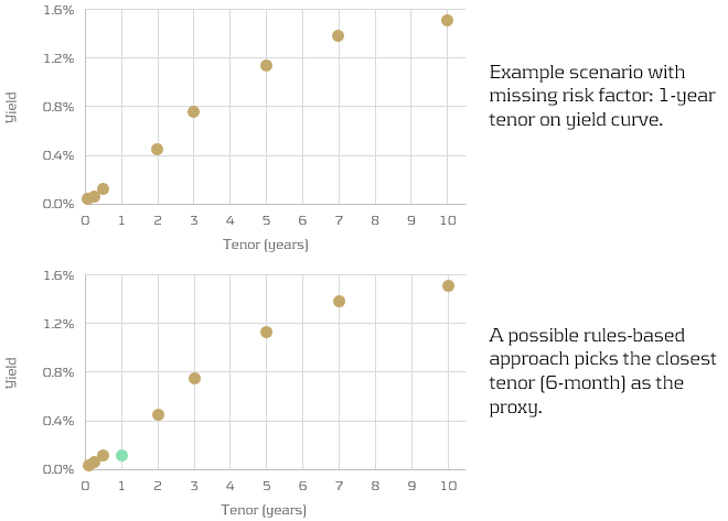
Rules-based approach

Rules-based approaches are more simplistic, however are less accurate than the statistical approaches. They find the “closest fit” modellable risk factor using somewhat more qualitative methods. For example, picking the closest tenor on a yield curve (see below), using relevant indices or ETFs, or limiting the search for proxies to the same sector as the underlying risk factor.

Similarly, longer tenor points (which may not be traded as frequently) can be decomposed into shorter-tenor points and cross-tenor basis spread.

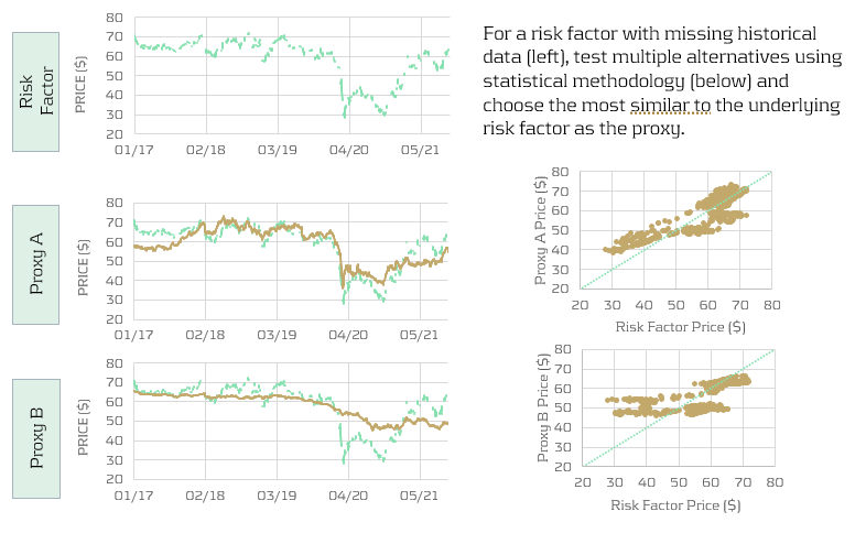
Statistical approach

Statistical approaches are more quantitate and more accurate than the rules-based approaches. However, this inevitably comes with computational expense. A large number of candidates are tested using the chosen statistical methodology and the closest is picked (see below).

For example, a regression approach could be used to identify which of the candidates are most correlated with the underlying risk factor. Studies have shown that statistical approaches not only produce the more accurate proxies, but can also reduce capital charges by almost twice as much as simpler rules-based approaches.

Conclusion

Risk factor modellability is a considerable concern for banks as it has a direct impact on the size of their capital charges. Inevitably, reducing the number of NMRFs is a key aim for all IMA banks. In this article, we show that developing proxies is one of the strategies that banks can use to minimise the amount of NMRFs in their models. Furthermore, we describe the two main approaches for developing proxies: rules-based and statistical. Although rules-based approaches are less complicated to develop, statistical approaches show much better accuracy and hence have the potential to better reduce capital charges.

Under the FRTB internal models approach (IMA), the capital calculation of risk factors is dependent on whether the risk factor is modellable. Insufficient data will result in more non-modellable risk factors (NMRFs), significantly increasing associated capital charges.

NMRFs

Risk factor modellability and NMRFs

The modellability of risk factors is a new concept which was introduced under FRTB and is based on the liquidity of each risk factor. Modellability is measured using the number of ‘real prices’ which are available for each risk factor. Real prices are transaction prices from the institution itself, verifiable prices for transactions between arms-length parties, prices from committed quotes, and prices from third party vendors.

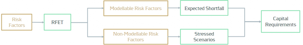
For a risk factor to be classed as modellable, it must have a minimum of 24 real prices per year, no 90-day period with less than four prices, and a minimum of 100 real prices in the last 12 months (with a maximum of one real price per day). The Risk Factor Eligibility Test (RFET), outlined in FRTB, is the process which determines modellability and is performed quarterly. The results of the RFET determine, for each risk factor, whether the capital requirements are calculated by expected shortfall or stressed scenarios.

Consequences of NMRFs for banks

Modellable risk factors are capitalised via expected shortfall calculations which allow for diversification benefits. Conversely, capital for NMRFs is calculated via stressed scenarios which result in larger capital charges. This is due to longer liquidity horizons and more prudent assumptions used for aggregation. Although it is expected that a low proportion of risk factors will be classified as non-modellable, research shows that they can account for over 30% of total capital requirements. 

There are multiple techniques that banks can use to reduce the number and impact of NMRFs, including the use of external data, developing proxies, and modifying the parameterisation of risk factor curves and surfaces. As well as focusing on reducing the number of NMRFs, banks will also need to develop early warning systems and automated reporting infrastructures to monitor the modellability of risk factors. These tools help to track and predict modellability issues, reducing the likelihood that risk factors will fail the RFET and increase capital requirements.

Methods for reducing the number of NMRFs

Banks should focus on reducing their NMRFs as they are associated with significantly higher capital charges. There are multiple approaches which can be taken to increase the likelihood that a risk factor passes the RFET and is classed as modellable.

Enhancing internal data

The simplest way for banks to reduce NMRFs is by increasing the amount of data available to them. Augmenting internal data with external data increases the number of real prices available for the RFET and reduces the likelihood of NMRFs. Banks can purchase additional data from external data vendors and data pooling services to increase the size and quality of datasets.

It is important for banks to initially investigate their internal data and understand where the gaps are. As data providers vary in which services and information they provide, banks should not only focus on the types and quantity of data available. For example, they should also consider data integrity, user interfaces, governance, and security. Many data providers also offer FRTB-specific metadata, such as flags for RFET liquidity passes or fails.

Finally, once a data provider has been chosen, additional effort will be required to resolve discrepancies between internal and external data and ensure that the external data follows the same internal standards.

Creating risk factor proxies

Proxies can be developed to reduce the number or magnitude of NMRFs, however, regulation states that their use must be limited. Proxies are developed using either statistical or rules-based approaches.

Rules-based approaches are simplistic, yet generally less accurate. They find the “closest fit” modellable risk factor using more qualitative methods, e.g. using the closest tenor on the interest rate curve. Alternatively, more accurate approaches model the relationship between the NMRF and modellable risk factors using statistical methods. Once a proxy is determined, it is classified as modellable and only the basis between it and the NMRF is required to be capitalised using stressed scenarios.

Determining proxies can be time-consuming as it requires exploratory work with uncertain outcomes. Additional ongoing effort will also be required by validation and monitoring units to ensure the relationship holds and the regulator is satisfied.

Developing own bucketing approach

Instead of using the prescribed bucketing approach, banks can use their own approach to maximise the number of real price observations for each risk factor.

For example, if a risk model requires a volatility surface to price, there are multiple ways this can be parametrised.  One method could be to split the surface into a 5x5 grid, creating 25 buckets that would each require sufficient real price observations to be classified as modellable. Conversely, the bank could instead split the surface into a 2x2 grid, resulting in only four buckets. The same number of real price observations would then need to be allocated between significantly less buckets, decreasing the chances of a risk factor being a NMRF.

It should be noted that the choice of bucketing approach affects other aspects of FRTB. Profit and Loss Attribution (PLA) uses the same buckets of risk factors as chosen for the RFET. Increasing the number of buckets may increase the chances of passing PLA, however, also increases the likelihood of risk factors failing the RFET and being classed as NMRFs.

Conclusion

In this article, we have described several potential methods for reducing the number of NMRFs. Although some of the suggested methods may be more cost effective or easier to implement than others, banks will most likely, in practice, need to implement a combination of these strategies in parallel. The modellability of risk factors is clearly an important part of the FRTB regulation for banks as it has a direct impact on required capital. Banks should begin to develop strategies for reducing the number of NMRFs as early as possible if they are to minimise the required capital when FRTB goes live.

The EBA has recently published the findings and observations from their TRIM on-site inspections. A significant number of deficiencies were identified and are required to be remediated by institutions in a timely fashion.

Since the Global Financial Crisis 2007-09, concerns have been raised regarding the complexity and variability of the models used by institutions to calculate their regulatory capital requirements. The lack of transparency behind the modelling approaches made it increasingly difficult for regulators to assess whether all risks had been appropriately and consistently captured.

The TRIM project was a large-scale multi-year supervisory initiative launched by the ECB at the beginning of 2016. The project aimed to confirm the adequacy and appropriateness of approved Pillar I internal models used by Significant Institutions (SIs) in euro area countries. This ensured their compliance with regulatory requirements and aimed to harmonise supervisory practices relating to internal models.

TRIM executed 200 on-site internal model investigations across 65 SIs from over 10 different countries. Over 5,800 deficiencies were identified. Findings were defined as deficiencies which required immediate supervisory attention. They were categorised depending on the actual or potential impact on the institution’s financial situation, the levels of own funds and own funds requirements, internal governance, risk control, and management.

The findings have been followed up with 253 binding supervisory decisions which request that the SIs mitigate these shortcomings within a timely fashion. Immediate action was required for findings that were deemed to take a significant time to address.

Assessment of Market Risk

TRIM assessed the VaR/sVaR models of 31 institutions. The majority of severe findings concerned the general features of the VaR and sVaR modelling methodology, such as data quality and risk factor modelling.

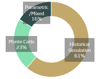
19 out of 31 institutions used historical simulation, seven used Monte Carlo, and the remainder used either a parametric or mixed approach. 17 of the historical simulation institutions, and five using Monte Carlo, used full revaluation for most instruments. Most other institutions used a sensitivities-based pricing approach.

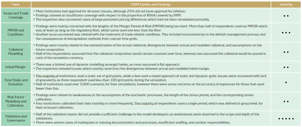
VaR/sVaR Methodology

Data: Issues with data cleansing, processing and validation were seen in many institutions and, on many occasions, data processes were poorly documented.

Risk Factors: In many cases, risk factors were missing or inadequately modelled. There was also insufficient justification or assessment of assumptions related to risk factor modelling.

Pricing: Institutions frequently had inadequate pricing methods for particular products, leading to a failure for the internal model to adequately capture all material price risks. In several cases, validation activities regarding the adequacy of pricing methods in the VaR model were insufficient or missing.

RNIME: Approximately two-thirds of the institutions had an identification process for risks not in model engines (RNIMEs). For ten of these institutions, this directly led to an RNIME add-on to the VaR or to the capital requirements.

Regulatory Backtesting

Period and Business Days: There was a lack of clear definitions of business and non-business days at most institutions. In many cases, this meant that institutions were trading on local holidays without adequate risk monitoring and without considering those days in the P&L and/or the VaR.

APL: Many institutions had no clear definition of fees, commissions or net interest income (NII), which must be excluded from the actual P&L (APL). Several institutions had issues with the treatment of fair value or other adjustments, which were either not documented, not determined correctly, or were not properly considered in the APL. Incorrect treatment of CVAs and DVAs and inconsistent treatment of the passage of time (theta) effect were also seen.

HPL: An insufficient alignment of pricing functions, market data, and parametrisation between the economic P&L (EPL) and the hypothetical P&L (HPL), as well as the inconsistent treatment of the theta effect in the HPL and the VaR, was seen in many institutions.

Internal Validation and Internal Backtesting

Methodology: In several cases, the internal backtesting methodology was considered inadequate or the levels of backtesting were not sufficient.

Hypothetical Backtesting: The required backtesting on hypothetical portfolios was either not carried or was only carried out to a very limited extent

IRC Methodology

TRIM assessed the IRC models of 17 institutions, reviewing a total of 19 IRC models. A total of 120 findings were identified and over 80% of institutions that used IRC models received at least one high-severity finding in relation to their IRC model. All institutions used a Monte Carlo simulation method, with 82% applying a weekly calculation. Most institutions obtained rates from external rating agency data. Others estimated rates from IRB models or directly from their front office function. As IRC lacks a prescriptive approach, the choice of modelling approaches between institutes exhibited a variety of modelling assumptions, as illustrated below.

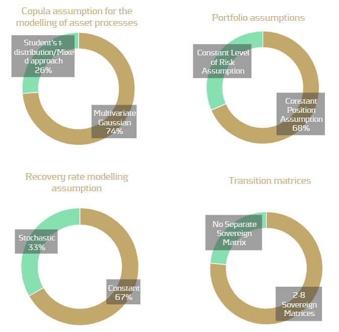
Recovery rates: The use of unjustified or inaccurate Recovery Rates (RR) and Probability of Defaults (PD) values were the cause of most findings. PDs close to or equal to zero without justification was a common issue, which typically arose for the modelling of sovereign obligors with high credit quality. 58% of models assumed PDs lower than one basis point, typically for sovereigns with very good ratings but sometimes also for corporates. The inconsistent assignment of PDs and RRs, or cases of manual assignment without a fully documented process, also contributed to common findings.

Modellingapproach: The lack of adequate modelling justifications presented many findings, including copula assumptions, risk factor choice, and correlation assumptions. Poor quality data and the lack of sufficient validation raised many findings for the correlation calibration.

Assessment of Counterparty Credit Risk

Eight banks faced on-site inspections under TRIM for counterparty credit risk. Whilst the majority of investigations resulted in findings of low materiality, there were severe weaknesses identified within validation units and overall governance frameworks.

Conclusion

Based on the findings and responses, it is clear that TRIM has successfully highlighted several shortcomings across the banks. As is often the case, many issues seem to be somewhat systemic problems which are seen in a large number of the institutions. The issues and findings have ranged from fundamental problems, such as missing risk factors, to more complicated problems related to inadequate modelling methodologies. As such, the remediation of these findings will also range from low to high effort. The SIs will need to mitigate the shortcomings in a timely fashion, with some more complicated or impactful findings potentially taking a considerable time to remediate.

Regulatory Landscape

Despite a delay of one year, many banks are struggling to be ready for FRTB in January 2023. Alongside the FRTB timeline, banks are also preparing for other important regulatory requirements and deadlines which share commonalities in implementation. We introduce several of these below.

SIMM

Initial Margin (IM) is the value of collateral required to open a position with a bank, exchange or broker.  The Standard Initial Margin Model (SIMM), published by ISDA, sets a market standard for calculating IMs. SIMM provides margin requirements for financial firms when trading non-centrally cleared derivatives.

BCBS 239

BCBS 239, published by the Basel Committee on Banking Supervision, aims to enhance banks’ risk data aggregation capabilities and internal risk reporting practices. It focuses on areas such as data governance, accuracy, completeness and timeliness. The standard outlines 14 principles, although their high-level nature means that they are open to interpretation.

SA-CVA

Credit Valuation Adjustment (CVA) is a type of value adjustment and represents the market value of the counterparty credit risk for a transaction. FRTB splits CVA into two main approaches: BA-CVA, for smaller banks with less sophisticated trading activities, and SA-CVA, for larger banks with designated CVA risk management desks.

IBOR

Interbank Offered Rates (IBORs) are benchmark reference interest rates. As they have been subject to manipulation and due to a lack of liquidity, IBORs are being replaced by Alternative Reference Rates (ARRs). Unlike IBORs, ARRs are based on real transactions on liquid markets rather than subjective estimates.

Synergies With Current Regulation

Existing SIMM and BCBS 239 frameworks and processes can be readily leveraged to reduce efforts in implementing FRTB frameworks.

SIMM

The overarching process of SIMM is very similar to the FRTB Sensitivities-based Method (SbM), including the identification of risk factors, calculation of sensitivities and aggregation of results. The outputs of SbM and SIMM are both based on delta, vega and curvature sensitivities. SIMM and FRTB both share four risk classes (IR, FX, EQ, and CM). However, in SIMM, credit is split across two risk classes (qualifying and non-qualifying), whereas it is split across three in FRTB (non-securitisation, securitisation and correlation trading). For both SbM and SIMM, banks should be able to decompose indices into their individual constituents. 

We recommend that banks leverage the existing sensitivities infrastructure from SIMM for SbM calculations, use a shared risk factor mapping methodology between SIMM and FRTB when there is considerable alignment in risk classes, and utilise a common index look-through procedure for both SIMM and SbM index decompositions.

BCBS 239

BCBS 239 requires banks to review IT infrastructure, governance, data quality, aggregation policies and procedures. A similar review will be required in order to comply with the data standards of FRTB. The BCBS 239 principles are now in “Annex D” of the FRTB document, clearly showing the synergy between the two regulations. The quality, transparency, volume and consistency of data are important for both BCBS 239 and FRTB. Improving these factors allow banks to easily follow the BCBS 239 principles and decrease the capital charges of non-modellable risk factors. BCBS 239 principles, such as data completeness and timeliness, are also necessary for passing P&L attribution (PLA) under FRTB.

We recommend that banks use BCBS 239 principles when designing the necessary data frameworks for the FRTB Risk Factor Eligibility Test (RFET), support FRTB traceability requirements and supervisory approvals with existing BCBS 239 data lineage documentation, and produce market risk reporting for FRTB using the risk reporting infrastructure detailed in BCBS 239.

Synergies With Future Regulation

The IBOR transition and SA-CVA will become effective from 2023. Aligning the timelines and exploiting the similarities between FRTB, SA-CVA and the IBOR transition will support banks to be ready for all three regulatory deadlines.

SA-CVA

Four of the six risk classes in SA-CVA (IR, FX, EQ, and CM) are identical to those in SbM. SA-CVA, however, uses a reduced granularity for risk factors compared to SbM. The SA-CVA capital calculation uses a similar methodology to SbM by combining sensitivities with risk weights. SA-CVA also incorporates the same trade population and metadata as SbM. SA-CVA capital requirements must be calculated and reported to the supervisor at the same monthly frequency as for the market risk standardised approach.

We recommend that banks combine SA-CVA and SbM risk factor bucketing tasks in a common methodology to reduce overall effort, isolate common components of both models as a feeder model, allowing a single stream for model development and validation, and develop a single system architecture which can be configured for either SbM or SA-CVA.

IBOR Transition

Although not a direct synergy, the transition from IBORs will have a direct impact to the Internal Models Approach (IMA) for FRTB and eligibility of risk factors. As the use of IBORs are discontinued, banks may observe a reduction in the number of real-price observations for associated risk factors due to a reduction in market liquidity. It is not certain if these liquidity issues fall under the RFET exemptions for systemic circumstances, which apply to modellable risk factors which can no longer pass the test. It may be difficult for banks to obtain stress-period data for ARRs, which could lead to substantial efforts to produce and justify proxies. The transition may cause modifications to trading desk structure, the integration of external data providers, and enhanced operational requirements, which can all affect FRTB.

We recommend that banks investigate how much data is available for ARRs, for both stress-period calculations and real-price observations, develop any necessary proxies which will be needed to overcome data availability issues, as soon as possible, and Calculate IBOR capital consequences through the existing FRTB engine.

Conclusion

FRTB implementation is proving to be a considerable workload for banks, especially those considering opting for the IMA. Several FRTB requirements, such as PLA and RFET, are completely new requirements for banks. As we have shown in this article, there are several other important regulatory requirements which banks are currently working towards. As such, we recommend that banks should leverage the synergies which are seen across this regulatory landscape to reduce the complexity and workload of FRTB.