
Financial institutions spend billions per year in their fight against fraud.
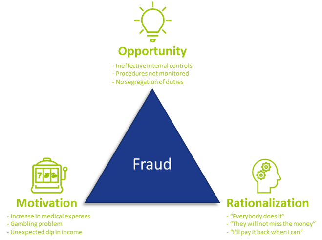
With every improvement, fraudsters look for and find new opportunities to exploit. When the opportunity arises, some people see a big incentive or pressure to commit fraud, and most will be able to justify to themselves why it is acceptable to commit fraud (as shown in the Fraud triangle – Figure 1). Unfortunately, the impact of fraud on organizations, individuals and society in general is substantial.
In a recent report by the Association of Certified Fraud Examiners (ACFE), Occupational Fraud 2022: A report to the nations, it is estimated that organizations lose about 5% of their revenue each year due to employees committing fraud against their employer. It is estimated that more than USD 4.7 trillion is lost worldwide to occupational fraud. Of these, most cases were identified through a tip to a hotline and most were not detected until 12 to 18 months later. The longer the fraud was undetected, the higher the loss. But organizations do not only fight fraud internally; external threats are also on the rise. As businesses evolve and processes are automated and digitalized, fraud activities become much more complex.
Data and modeling approach to fraud prevention
To effectively prevent fraud, it first needs to be identified. Traditionally, employees are trained to identify anomalies or inconsistencies in their daily work environment. It is still crucial that your employees know what to look for and how to spot suspicious activities. But due to the complexities and vast amounts of information available, and because fraudsters are becoming more sophisticated, it becomes much more difficult to determine whether a potential customer is a fraudster or a real client.
The good news is that digitalization and increased data availability provides the opportunity for data analytics. It is important to note here that it does not completely replace your current processes; it should be used in addition to your traditional prevention and/or detection methods to be more effective to proactively identify and prevent fraud in your organization.
Benefits of data analytics
Traditionally, sampling was done on a population to test for fraud instances, but this may not be as effective because it only looks at a small population. Because fraud numbers reported usually being small (but with a large monetary impact), it is possible to overlook valuable insights if only samples of populations are investigated. Ideally, all data should be included to identify trends and potential fraudulent activities, and with data analytics that is possible. By analyzing large amounts of data, organizations can identify patterns and trends that may indicate fraudulent activity. It can help to improve the accuracy of fraud detection systems, as they can be trained to recognize these patterns.
Data analytics can increase efficiency by reducing false positives and false negatives and assists organizations to automate parts of the fraud detection processes, which can save time and resources. This allows the business to focus on other important strategic objectives and tasks such as customer service and product development.
By using data analytics to identify and prevent fraudulent activity, organizations can help to protect their customers against financial losses and other harm. Customer trust and loyalty are built when organizations show they are serious about the welfare and safety of their customers.
Detecting and preventing fraud
Reality is that preventing fraud upfront or in an early stage is much more economical and beneficial than having to detect fraud after the fact, as investigations are time-consuming and the fraud is not always easy to proof in court. Moreover, by the time it is detected, a loss may have already been incurred. Using data analytics to identify fraudsters and fraudulent activities earlier, can protect the bottom line by reducing financial losses and improving the organization’s overall financial performance.
By using analytics to detect and prevent fraud, organizations can demonstrate to regulatory bodies that they are taking compliance seriously. Reporting suspicious transactions and activities to regulatory bodies is a key component of complying with anti-money laundering and counter-terrorism financing legislation, and analytics can assist with identifying these transactions and activities more effectively.
Data analytics can be used to prevent fraud at onboarding, detect it in the existing customer base, and to make your operational processes more efficient. More specifically, data analytics can be used and leveraged as follows:
- Identifying outlier trends and hidden patterns can highlight areas and/or transactions that are more vulnerable to fraud.
- Automating identification of exceptions removes manual intervention and makes the identification criteria more consistent.
- Traditional physical reviews using limited resources to investigate is time-consuming. Data analytics can be used to prioritize the ones with the highest impact and risk, e.g. investigate the suspicious transactions with the highest value first.
- Combining data from different data sources to feed into a model provides a more holistic view of a customer or scenario than looking at individual transactions or applications in isolation.
- Both structured and unstructured data can be used to prevent and detect fraud.
- Fraud propensity model scoring can run automatically and generate results to be reviewed and investigated in real-time or near real-time.
- Analyzing relationships between various entities and customers using Social Network Analysis (SNA). Traditionally, networks/links were identified by the investigator while building a case. By using analytics, less time is needed to identify these relationships. Also, it identifies valuable links previously unknown, as additional levels of relationships can be examined.
- Specific modus operandi identified by the organization’s internal fraud team can be translated into data models to automate identification of similar cases. (See Case study below)
- Applying a fraud model to the organization’s bad debt book can assist with your collections strategy. Fraudsters never intended to pay and focusing your collection efforts on them wastes time and valuable resources. Most efforts should be on those cases where money can be collected.
Case study
The Zanders data analytics team has experience with applying data analytics within a company to identify customers who create synthetic profiles at point of application. By working closely with investigators, a model was developed in which one out of every three applications referred for investigation was classified as fraudulent.
The benefit of introducing analytics was twofold – from an onboarding- and existing customer point of view. The number of fraudsters identified before onboarding increased, preventing (potential) losses. Using the positive identified frauds at point of application, and checking the profile against the existing book, helped to identify areas that were more vulnerable where investigation should be prioritized.
The project proved that:
- Data analytics is valuable and combining it with insights from the operational teams is powerful.
- The buy-in from the stakeholders made the model more effective. If the team investigating the alert does not trust the model or does not know what to look for, there will be resistance in investigating the alerts.
- Taking your internal fraud team on a data and analytics journey is a must. They need to understand the impact that their decisions and captured outcomes can have on future models.
- Challenges with false positives (within business appetite and investigation capacity) are a reality, but having a model is better than searching for a needle in a haystack. Learning from the results and outcomes of the investigations, even if they were false positives, will enhance your next model.
- One size does not fit all. Fraud models need to be tailored to the business’ needs.
Conclusion
While using data analytics to identify fraudulent activities is an investment, organizations need to outweigh the benefit of incorporating data analytics in their current processes against the potential losses. Fraud not only results in monetary losses, it can lead to reputational damage and have an impact on the organization’s market share as customers will not do business with an organization where they don’t feel protected. Your customers also expect great customer service and implementing proactive fraud prevention measures increases confidence in your organization.
How can Zanders help your organization?
Did you find this article helpful but do you still have questions or need additional assistance? Our team of experts is ready to assist you in finding the solutions you need. Please feel free to reach out to us to discuss your needs in more detail. Whether you’re looking for advice on a specific project or just need someone to exchange ideas with, we are here to assis

In March 2021, the European Banking Authority (EBA) was mandated through Article 501c of the Capital Requirements Regulation (CRR) to “assess […] whether a dedicated prudential treatment of exposures related to assets or activities associated substantially with environmental and/or social objectives would be justified”.
More simply put, the EBA was asked to investigate whether the current prudential framework properly captures environmental and social risks. In response, the EBA published a Discussion Paper (DP) [1] in May 2022 to collect input from stakeholders such as academia and banking professionals.
After briefly presenting the DP, this article reviews the current Pillar 1 Capital (P1C) requirements. We limit ourselves to the P1C requirements for credit risk as this is by far the largest risk type for banks. Furthermore, we only discuss the interaction of the P1C with climate change risks (as opposed to broader environmental and/or social risk types). After establishing the extent to which the prudential framework takes climate change risks into account, possible amendments to the framework will be considered.
Key take-aways of this article:
- The current prudential framework includes several mechanisms that allow the reflection of climate change risks into the P1C.
- The interaction between P1C and climate change risks is limited to specific parts of the portfolio, and in those cases, it remains to be seen to what extent this is properly accounted for at the moment.
- Amendments to the prudential framework can be considered, but it is important to avoid double counting issues and to take into account differences in time horizons.
- The EBA is expected to publish a final report on the prudential treatment of environmental risks in the first half of this year.
- Financial institutions that are using the internal ratings-based approach are advised to start with the incorporation of climate change risks into PD and LGD models.
EBA’s Discussion Paper

In the introduction of the DP, the EBA mentions the increasing environmental risks – and their interaction with the traditional risk types – as the trigger for the review of the prudential framework. One of the main concerns is whether the current framework is sufficiently capturing the impact of transition risks and the more frequent and severe physical risks expected in the coming decades. In this context, they stress the special characteristics of environmental risks: compared to the traditional risk types, environmental risks tend to have a “multidimensional, non-linear, uncertain and forward-looking nature.”
The EBA also explains that the P1C requirements are not intended to cover all risks a financial institution is exposed to. The P1C represents a baseline capital requirement that is complemented by the Pillar 2 Capital requirement, which is more reflective of a financial institution’s specific business model and risks. Still, it is warranted to assess whether environmental risks are appropriately reflected in the P1C requirements, especially if these lead to systemic risks.
Even though the DP raises more questions than it provides answers, some starting points for the discussion are introduced. One is that the EBA takes a risk-based approach. Their standpoint is that changes to the prudential framework should reflect actual risk differentials compared to other risk types and that it should not be a tool to (unjustly) incentivize the transition to a sustainable economy. The latter lies “in the remit of political authorities.”
The DP also discusses some challenges related to environmental risks. One example is the lack of high-quality, granular historical data, which is needed to support the calibration of the prudential framework. The EBA also mentions the mismatch in the time horizon for the prudential framework (i.e., a business cycle) and the time horizon over which the environmental risks will unfold (i.e., several decades). They wonder whether “the business cycle concepts and assumptions that are used in estimating risk weights and capital requirements are sufficient to capture the emergence of these risks.”
Finally, the EBA does not favor supporting and/or penalizing factors, i.e., the introduction of adjustments to the existing risk weights based on a (green) taxonomy-based classification of the exposures1. They are right to argue that there is no direct relationship between an exposure’s sustainability profile and its credit risk. In addition, there is a risk of double counting if environmental risk drivers have already been reflected in the current prudential framework. Consequently, the EBA concludes that targeted amendments to the framework may be more appropriate. An example would be to ensure that environmental risks are properly included in external credit ratings and the credit risk models of financial institutions. We explain this in more detail in the following paragraphs.
Pillar 1 Capital requirements
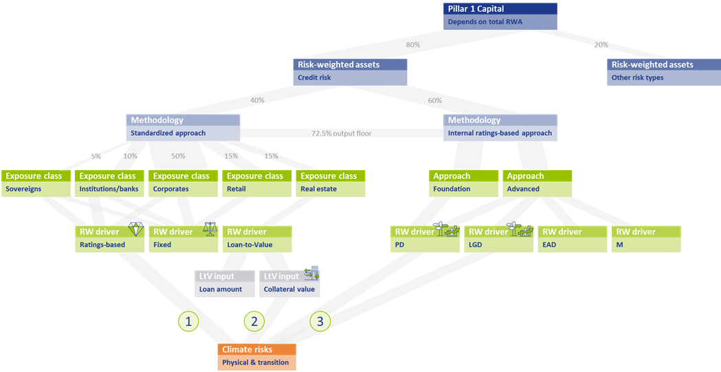
The assessment to what extent climate change risks are properly captured in the current prudential framework requires at least a high-level understanding of the framework. Figure 1 presents a schematic overview of the P1C requirements.
The P1C (at the top of Figure 1) depends on the total amount of Risk-Weighted Assets (RWAs; on the row below)2. RWAs are determined separately for each (traditional) risk type. As mentioned, we only focus on credit risk in this article. The RWAs for credit risk are approximately 80% of the average bank’s total RWAs3. Financial institutions can choose between two methodologies for determining their credit risk RWAs: the Standardized Approach (SA)4 and the internal ratings-based (IRB) approach5 . In Europe, on average 40% of the total RWAs for credit risk are based on the SA, while the rest is based on the IRB approach6 :
Figure 1 – Schematic overview of the P1C requirements and the interaction with climate change risks
Standardized Approach
In the SA, risk weights (RWs) are assigned to individual exposures, depending on their exposure class. About 50% of the RWAs for credit risk in the SA stem from the Corporates exposure class7. Generally speaking, there are three possible RW drivers: the RWAs depend on the external credit rating for the exposure, a fixed RW applies, or the RW depends on the Loan-to-Value8 (LtV) of the (real estate) exposure. The RW for an exposure to a sovereign bond for example, is either equal to 100% if no external credit rating is available (a fixed RW) or it ranges between 0% (for an AAA to AA-rated bond) and 150% (for a below B-rated bond).
Internal Ratings-Based Approach
Within the IRB approach, a distinction is made between Foundation IRB (F-IRB) and Advanced IRB (A-IRB). In both cases, a financial institution is allowed to use its internal models to determine the Probability of Default (PD) for the exposure. In the A-IRB approach, the financial institution in addition is allowed to use internal models to determine the Loss Given Default (LGD), Exposure at Default (EAD), and the Effective Maturity (M).
Interaction with climate change risks
The overview of the P1C requirements introduced in the previous section allows us to investigate the interaction between climate change risks and the P1C requirement. This is done separately for the SA and the IRB approach.
Standardized Approach
In the SA, there are two elements that allow for interaction between climate change risks and the resulting P1C. Climate change risks could be reflected in the P1C if the RW depends on an external credit rating, and this rating in turn properly accounts for climate change risks in the assessment of the counterparty’s creditworthiness (see 1 in Figure 1). The same holds if the RW depends on the LtV and in turn, the collateral valuation properly accounts for climate change risks (see 2 in Figure 1). This raises several concerns:

First, it can be questioned whether external credit ratings are properly capturing all climate change risks. In a report from the Network for Greening the Financial System (NGFS) [3], which was published at the same time as EBA’s DP, it is stated that credit rating agencies (CRAs) have so far not attempted to determine the credit impact of environmental risk factors (through back-testing for example). Also, the lack of high-quality historical data is mentioned as an explanation that statistical relationships between environmental risks and credit ratings have not been quantified. Further, a paper published by the ECB [4] concludes that, given the current level of disclosures, it is impossible for users of credit ratings to establish the magnitude of adjustments to the credit rating stemming from ESG-related risks. Nevertheless, they state that credit rating agencies “have made significant progress with their disclosures and methodologies around ESG in recent years.” The need for this is supported by academic research. An example is a study [5] from 2021 in which a correlation between credit default swap (CDS) spreads and ESG performance was demonstrated, and a study from 2020 [6] which demonstrated that high emitting companies have a shorter distance-to-default.

Secondly, the EBA has reported in the DP that less than 10% of the SA’s total RWAs is derived based on external credit ratings. This implies that a large share of the total RWAs is assigned a fixed RW. Obviously, in those cases there is no link between the P1C and the climate change risks involved in those exposures.

Finally, climate change risks only impact the P1C maintained for real estate exposures to the extent that these risks have been reflected in collateral valuations. Although climate change risks are priced in financial markets according to academic literature, many papers and institutions indicate that these risks are not (yet) fully reflected. In a survey held by Stroebel and Wurgler in 2021 [7], it is shown that a large majority of the respondents (consisting of finance academics, professionals and public sector regulators, among others) is of the opinion that climate change risks have insufficiently been priced in financial markets. A nice overview of this and related literature is presented in a publication from the Bank for International Settlements (BIS) [8]. The EBA DP itself lists some research papers in chapter 5.1 that indicate a relationship between a home’s sales price and its energy efficiency, or with the occurrence of physical risk events. It is unclear though if climate change risks are fully captured in the collateral valuations. For example, research is presented that information on flood risk is not priced into residential property prices. Recent research by ABN AMRO [9] also shows this.
Internal Ratings-Based Approach
In the IRB approach, financial institutions have more flexibility to include climate change risks in their internal models (see 3 in Figure 1). In the F-IRB approach this is limited to PD models, but in the A-IRB approach also LGD models can be adjusted.

A complicating factor is the forward-looking nature of climate change risks. In recent years, the competent authorities have pressured financial institutions to use historical data as much as possible in their model calibration and to back-test the performance of their models. As climate change risks will unfold over the next couple of decades, these are not (yet) reflected in historical data. To incorporate climate change risk, expert judgement would therefore be required. This has been discouraged over the past years (e.g., through the ECB’s Targeted Review of Internal Models (TRIM)) and it will probably trigger a discussion with the competent authorities. A possible deterioration of model performance (due to higher estimated risks compared to historically observations) is just one example that may attract attention.

Another complicating factor is that under the IRB approach, the PD of an obligor is estimated based on long-run average one-year default rates. While this may be an appropriate approach if there are no clear indications that the overall risk level will change, this does not hold if climate change risks increase in the future, and possibly increase systemic risks. By continuing to base a PD model on historical data only, especially for exposures with a time to maturity beyond a couple of years, the credit risk may be understated.
Are amendments to the prudential framework needed?
We have explained that there are several mechanisms in the prudential framework that allow environmental risks to be included in the P1C: the use of external credit ratings, the valuation of collateral, and the PD and LGD models used in the IRB approach. We have also seen, however, that it is questionable whether these mechanisms are fully effective. External credit ratings may not properly reflect all environmental risks and these risks may not be fully priced in on capital markets, leading to incorrect collateral values. Finally, a large share of the RWAs for credit risk depends on fixed RWs that are not (environmentally) risk-sensitive.
Consequently, it can be argued that amendments or enhancements to the prudential framework are needed. One must be careful, however, as the risk of double counting is just around the corner. Therefore, the following amendments or actions should be considered:
- Further research should be undertaken to investigate the relationship between climate change risk and the creditworthiness of counterparties. If there is more clarity on this relationship, it should also be assessed to what extent this relationship is sufficiently reflected in external ratings. Requiring more advanced disclosures from credit rating agencies could help to understand whether these risks are sufficiently captured in the prudential framework. One should be cautious to amend the ratings-based RWs in the SA, since credit rating agencies are continuously working on the inclusion of environmental risks into their credit assessments; there would be a real risk of double counting.
- The potential negative impact of climate change risks on collateral value should be further investigated. Financial institutions are already required by the ECB9 to consider environmental risks in their collateral valuations but this is not at a sufficient level yet. It will be important to consider the possibility of sudden value changes due to transition risks like shifting consumer sentiment or awareness.
- To improve the risk-sensitivity of the framework, a dependency on the carbon emissions of the counterparty could be introduced in the fixed RWs, possibly only for the most carbon-intensive sectors. It could be argued that there are other factors that have a more significant relationship with the default risk of a certain counterparty that could be included in the SA. Climate change risks, however, differ in the sense that they can lead to a systemic risk (as opposed to an idiosyncratic risk) that is currently not captured in the overall level of the RWs.
- In the SA, a distinction could be introduced based on the exposure’s time to maturity. For relatively short-term exposures, the current calibrations are probably fine. For longer-term exposures, however, the risks stemming from climate change may be underestimated as these are expected to increase over time.
- In the IRB approach, a reflection of climate change risk would require the regulator to allow for forward-looking expert judgment in the (re)calibration of PD and LGD models. Further guidance from the competent authorities on the potentially negative impact on model performance based on historical data would also be useful.
Conclusion
Based on the schematic overview of the P1C requirements and the (potential) interaction with climate change risks, we conclude that several mechanisms in the prudential framework allow for climate change risks to be incorporated into the P1C. At the same time, we conclude that this interaction is limited to specific parts of the portfolio, and that in those cases it remains to be seen to what extent this is properly accounted for. To remedy this, amendments to the prudential framework could be considered. It is important, however, to avoid double counting issues and to be mindful of time horizon differences.
It is expected that the EBA will publish a final report on the prudential treatment of environmental risks in the first half of this year. However, especially financial institutions that are using the IRB approach should not take a wait-and-see approach. Given the complexity of modeling climate change risks, it is prudent to start incorporating climate change risks into PD and LGD models sooner rather than later.
With Zanders’ extensive experience covering both credit risk modeling and climate change risk, we are well suited to support with this process. If you are looking for support, please reach out to us.
1 Supporting factors are currently in place for SMEs and infrastructure projects, but the EBA advocated their removal.
2 See RBC20.1 in the Basel Framework.
3 See for example the results from the EBA’s EU-wide transparency exercise. This is reflected in Figure 1 by the percentage in the grey link between P1C and RWAs for credit risk.
4 See CRE20 to CRE22 in the Basel Framework.
5 See CRE30 to CRE36 in the Basel Framework.
6 In the Netherlands, less than 20% of the total RWAs is based on the SA. See the EBA’s EU-wide transparency exercise for more information. The percentages in the grey link between ‘Risk-weighted assets’ and ‘Methodology’ in Figure 1 are based on the European average.
7 See the EBA’s Risk assessment of the European banking system [2]. The percentages in the grey link between ‘Standardized Approach’ and the ‘Exposure class’ in Figure 1 reflect the share of RWAs in the SA for each of the different exposure classes.
8 The LtV is defined as the ratio between the loan amount and the value of the property that serves as collateral.
9 See expectation 8.3 in the ECB’s Guide on climate-related and environmental risks.
References
- The role of environmental risks in the prudential framework, European Banking Authority, Discussion Paper, 2 May 2022
- Risk assessment of the European banking system, European Banking Authority, December 2022
- Capturing risk differentials from climate-related risks, Network for Greening the Financial System, Progress Report, May 2022
- Disclosure of climate change risk in credit ratings, European Central Bank, Occasional Paper Series, No. 303, September 2022
- Pricing ESG risk in credit markets, Federated Hermes, March 2021
- Climate change and credit risk, Capasso, Gianfrate, and Spinelli, Journal of Cleaner Production, Volume 266, September 2020
- What do you think about climate finance?, Stroebel and Wurgler, Journal of Financial Economics, vol 142, no 2, November 2021
- Pricing of climate risks in financial markets, Bank for International Settlements, Monetary and Economic Department, December 2022
- Is flood risk already affecting house prices?, ABN AMRO, 11 February 2022
- Guide on climate-related and environmental risks, European Central Bank, November 2020

Increasing Shareholder Value by Utilizing Tax Opportunities
The WACC is a calculation of the ‘after-tax’ cost of capital where the tax treatment for each capital component is different. In most countries, the cost of debt is tax deductible while the cost of equity isn’t, for hybrids this depends on each case.
Some countries offer beneficial tax opportunities that can result in an increase of operational cash flows or a reduction of the WACC.
This article elaborates on the impact of tax regulation on the WACC and argues that the calculation of the WACC for Belgian financing structures needs to be revised. Furthermore, this article outlines practical strategies for utilizing tax opportunities that can create shareholder value.
The eighth and last article in this series on the weighted average cost of capital (WACC) discusses how to increase shareholder value by utilizing tax opportunities. Generally, shareholder value can be created by either:
- Increasing operational cash flows, which is similar to increasing the net operating profit ‘after-tax’ (NOPAT);
- or Reducing the ‘after-tax’ WACC.
This article starts by focusing on the relationship between the WACC and tax. Best market practice is to reflect the actual environment in which a company operates, therefore, the general WACC equation needs to be revised according to local tax regulations. We will also outline strategies for utilizing tax opportunities that can create shareholder value. A reduction in the effective tax rate and in the cash taxes paid can be achieved through a number of different techniques.
Relationship Between WACC and Tax
Within their treasury and finance activities, multinational companies could trigger a number of different taxes, such as corporate income tax, capital gains tax, value-added tax, withholding tax and stamp or capital duties. Whether one or more of these taxes will be applicable depends on country specific tax regulations. This article will mainly focus on corporate tax related to the WACC. The tax treatment for the different capital components is different. In most countries, the cost of debt is tax deductible while the cost of equity isn’t (for hybrids this depends on each case).
The corporate tax rate in the general WACC equation, discussed in the first article of this series (see Part 1: Is Estimating the WACC Like Interpreting a Piece of Art?), is applicable to debt financing. It is appropriate, however, to take into consideration the fact that several countries apply thin capitalization rules that may restrict tax deductibility of interest expenses to a maximum leverage.
Furthermore, in some countries, expenses on hybrid capital could be tax deductible as well. In this case the corporate tax rate should also be applied to hybrid financing and the WACC equation should be changed accordingly.
Finally, corporate tax regulation can also have a positive impact on the cost of equity. For example, Belgium has recently introduced a system of notional interest deduction, providing a tax deduction for the cost of equity (this is discussed further in the section below: Notional Interest Deduction in Belgium).
As a result of the factors discussed above, we believe that the ‘after-tax’ capital components in the estimation of the WACC need to be revised for country specific tax regulations.
Revised WACC Formula
In other coverage of this subject, a distinction is made between the ‘after-tax’ and ‘pre-tax’ WACC, which is illustrated by the following general formula:
WACCPT = WACCAT / [1 – TC]
WACCAT : Weighted average cost of capital after-tax
WACCPT : Weighted average cost of capital pre-tax
TC : Corporate income tax rate
In this formula the ‘after-tax’ WACC is grossed-up by the corporate tax rate to generate the ‘pre-tax’ WACC. The correct corporate tax rate for estimating the WACC is the marginal tax rate for the future! If a company is profitable for a long time into the future, then the tax rate for the company will probably be the highest marginal statutory tax rate.
However, if a company is loss making then there are no profits against which to offset the interest. The effective tax rate is therefore uncertain because of volatility in operating profits and a potential loss carry back or forward. For this reason the effective tax rate may be lower than the statutory tax rate. Consequently, it may be useful to calculate multiple historical effective tax rates for a company. The effective tax rate is calculated as the actual taxes paid divided by earnings before taxes.
Best market practice is to calculate these rates for the past five to ten years. If the past historical effective rate is lower than the marginal statutory tax rate, this may be a good reason for using that lower rate in the assumptions for estimating the WACC.
This article focuses on the impact of corporate tax on the WACC but in a different way than previously discussed before. The following formula defines the ‘after-tax’ WACC as a combination of the WACC ‘without tax advantage’ and a ‘tax advantage’ component:
WACCAT = WACCWTA – TA
WACCAT : Weighted average cost of capital after-tax
WACCWTA : Weighted average cost of capital without tax advantage
TA : Tax advantage related to interest-bearing debt, common equity and/or hybrid capital
Please note that the ‘pre-tax’ WACC is not equal to the WACC ‘without tax advantage’. The main difference is the tax adjustment in the cost of equity component in the pre-tax calculation. As a result, we prefer to state the formula in a different way, which makes it easier to reflect not only tax advantages on interestbearing debt, but also potential tax advantages on common equity or hybrid capital.
The applicable tax advantage component will be different per country, depending on local tax regulations. An application of this revised WACC formula will be further explained in a case study on notional interest deduction in Belgium.
Notional Interest Deduction in Belgium
Recently, Belgium introduced a system of notional interest deduction that provides a tax deduction for the cost of equity. The ‘after-tax’ WACC formula, as mentioned earlier, can be applied to formulate the revised WACC equation in Belgium:
WACCAT = WACCWTA – TA
WACCWTA : Weighted average cost of capital without tax advantage, formulated as follows: RD x DM / [DM+EM] + RE x EM / [DM+EM] TA : Tax advantage related to interest-bearing debt and common equity, formulated as follows: TC x [RD x DM + RN x EB] / [DM+EM] TC : Corporate tax rate in Belgium
RD : Cost of interest-bearing debt
RE : Cost of common equity
RN : Notional interest deduction
DM : Market value of interest-bearing debt
EM : Market value of equity
EB : Adjusted book value of equity
The statutory corporate tax rate in Belgium is 33.99%. The revised WACC formula contains an additional tax deduction component of [RN x EB], which represents a notional interest deduction on the adjusted book value of equity. The notional interest deduction can result in an effective tax rate, for example, intercompany finance activities of around 2-6%.
The notional interest is calculated based on the annual average of the monthly published rates of the long-term Belgian government bonds (10-year OLO) of the previous year. This indicates that the real cost of equity, e.g. partly represented by distributed dividends, is not deductible but a notional risk-free component.
The adjusted book value of equity qualifies as the basis for the tax deduction. The appropriate value is calculated as the total equity in the opening balance sheet of the taxable period under Belgian GAAP, which includes retained earnings, with some adjustments to avoid double use and abuse. This indicates that the value of equity, as the basis for the tax deduction, is not the market value but is limited to an adjusted book value.
As a result, Belgium offers a beneficial tax opportunity that can result in an increase of shareholder value by reducing the ‘after-tax’ WACC. Belgium is, therefore, on the short-list for many companies seeking a tax-efficient location for their treasury and finance activities. Furthermore, the notional interest deduction enables strategies for optimizing the capital structure or developing structured finance instruments.
How to Utilize Tax Opportunities?
This article illustrates the fact that managing the ‘after-tax’ WACC is a combined strategy of minimizing the WACC ‘without tax advantages’ and, at the same time, maximizing tax advantages. A reduction in the effective tax rate and in the cash taxes paid can be achieved through a number of different techniques. Most techniques have the objective to obtain an interest deduction in one country, while the corresponding income is taxed at a lower rate in another country. This is illustrated by the following two examples.
The first example concerns a multinational company that can take advantage of a tax rate arbitrage obtained through funding an operating company from a country with a lower tax rate than the country of this operating company. For this reason, many multinational companies select a tax-efficient location for their holding or finance company and optimize their transfer prices.
Secondly, country and/or company specific hybrid capital can be structured, which would be treated differently by the country in which the borrowing company is located than it would be treated by the country in which the lending company is located. The potential advantage of this strategy is that the expense is treated as interest in the borrower’s country and is therefore deductible for tax purposes.
However, at the same time, the country in which the lender is located would treat the corresponding income either as a capital receipt, which is not taxable or it can be offset by capital losses or other items; or as dividend income, which is either exempt or covered by a credit for the foreign taxes paid. As a result, it is beneficial to optimize the capital structure and develop structured finance instruments.
There is a range of different strategies that may be used to achieve tax advantages, depending upon the particular profile of a multinational company. Choosing the strategy that will be most effective depends on a number of factors, such as the operating structure, the tax profile and the repatriation policy of a company. Whatever strategy is chosen, a number of commercial aspects will be paramount. The company will need to align its tax planning strategies with its business drivers and needs.
The following section highlights four practical strategies that illustrate how potential tax advantages and, as a consequence, an increase in shareholder value can be achieved by:
- Selecting a tax-efficient location.
- Optimizing the capital structure.
- Developing structured finance instruments.
- Optimizing transfer prices.
Selecting a tax-efficient location
Many companies have centralized their treasury and finance activities in a holding or separate finance company. Best market practice is that the holding or finance company will act as an in-house bank to all operating companies. The benefit of a finance company, in comparison to a holding, is that it is relatively easy to re-locate to a tax-efficient location. Of course, there are a number of tax issues that affect the choice of location. Selecting an appropriate jurisdiction for the holding or finance company is critical in implementing a tax-efficient group financing structure.
Before deciding to select a tax-efficient location, a number of issues must be considered. First of all, whether the group finance activities generate enough profit to merit re-locating to a low-tax jurisdiction. Secondly, re-locating activities affects the whole organization because it is required that certain activities will be carried out at the chosen location, which means that specific substance requirements, e.g. minimum number of employees, have to be met. Finally, major attention has to be paid to compliance with legal and tax regulation and a proper analysis of tax-efficient exit strategies. It is advisable to include all this information in a detailed business case to support decision-making.
When selecting an appropriate jurisdiction, several tax factors should be considered including, but not limited to, the following: The applicable taxes, the level of taxation and the availability of special group financing facilities that can reduce the effective tax rate.
- The availability of tax rulings to obtain more certainty in advance.
- Whether the jurisdiction has an expansive tax treaty network.
- Whether dividends received are subject to a participation exemption or similar exemption.
- Whether interest payments are restricted by a thin capitalization rule.
- Whether a certain controlled foreign company (CFC) rule will absorb the potential benefit of the chosen jurisdiction.
Other important factors include the financial infrastructure, the availability of skilled labor, living conditions for expatriates, logistics and communication, and the level of operating costs.
Based on the aforementioned criteria, a selection of attractive countries for locating group finance activities is listed below:
Belgium: In 2006, Belgium introduced a notional interest deduction as an alternative for the ‘Belgian Co-ordination Centres’. This regime allows taxefficient equity funding of Belgian resident companies and Belgian branches of non-resident companies. As a result, the effective tax rate may be around 2-6%.
Ireland: Ireland has introduced an attractive alternative to the previous ‘IFSC regime’ by lowering the corporate income tax rate for active trading profits to 12.5%. Several treasury and finance activities can be structured easily to generate active trading profit taxed at this low tax rate.
Switzerland: Using a Swiss finance branch structure can reduce the effective tax rate here. These structures are used by companies in Luxembourg. The benefits of this structure include low taxation at federal and cantonal level based on a favorable tax ruling – a so called tax holiday – which may reduce the effective tax rate to even less than 2%.
The Netherlands: Recently, the Netherlands proposed an optional tax regulation, the group interest box, which is a special regime for the net balance of intercompany interest within a group, taxed at a rate of 5%. This regulation should serve as a substitute for the previous ‘Dutch Finance Company’.
Optimizing the capital structure
One way to achieve tax advantages is by optimizing not only the capital structure of the holding or finance company but that of the operating companies as well. Best market practice is to take into account the following tax elements:
Thin capitalization: When a group relationship enables a company to take on higher levels of debt than a third party would lend, this is called thin capitalization. A group may decide to introduce excess debt for a number of reasons. For example, a holding or finance company may wish to extract profits tax-efficiently, or may look to increase the interest costs of an operating company to shelter taxable profits.
To restrict these situations, several countries have introduced thin capitalization rules. These rules can have a substantial impact on the deductibility of interest on intercompany loans.
Withholding tax: Interest and dividend payments can be subject to withholding tax, although in many countries dividends are exempt from withholding tax. As a result, high rates of withholding tax on interest can make traditional debt financing unattractive. However, tax treaties can reduce withholding tax. As a consequence, many companies choose a jurisdiction with a broad network of tax treaties.
Repatriation of cash: If a company has decided to centralize its group financing, then it is relevant to repatriate cash that can be used for intercompany financing. In most countries, repatriation of cash can be performed through dividends, intercompany loans or back-to-back loans. It depends on each country what will be the most tax-efficient method.
Developing structured finance instruments
Developing structured finance instruments can be interesting for funding or investment activities. Examples of structured finance instruments are:
Hybrid capital instruments: Hybrid capital combines certain elements of debt and equity. Examples are preferred equity, convertible bonds, subordinated debt and index-linked bonds. For the issuers, hybrid securities can combine the best features of both debt and equity: tax deductibility for coupon payments, reduction in the overall cost of capital and strengthening of the credit rating.
Tax sparing investment products: To encourage investments in their countries, some countries forgive all or part of the withholding taxes that would normally be paid by a company. This practice is known as tax sparing. Certain tax treaties consider spared taxes as having been paid for purposes of calculating foreign tax deductions and credits. This is, for example, the case in the tax treaty between The Netherlands with Brazil, which enables the structuring of tax-efficient investment products.
Double-dip lease constructions: A double-dip lease construction is a cross-border lease in which the different rules of the lessor’s and lessee’s countries let both parties be treated as the owner of the leased equipment for tax purposes. As a result of this, a double interest deduction is achieved, also called double dipping.
Optimizing transfer prices
Transfer pricing is generally recognized as one of the key tax issues facing multinational companies today. Transfer pricing rules are applicable on intercompany financing activities and the provision of other treasury and finance services, e.g. the operation of cash pooling arrangements or providing hedging advice.
Currently, in many countries, tax authorities require that intercompany loans have terms and conditions on an arm’s length basis and are properly documented. However, in a number of countries, it is still possible to agree on an advance tax ruling for intercompany finance conditions.
Several companies apply interest rates on intercompany loans, being the same rate as an external loan or an average rate of the borrowings of the holding or finance company. When we apply the basic condition of transfer pricing to an intercompany loan, this would require setting the interest rate of this loan equal to the rate at which the borrower could raise debt from a third party.
In certain circumstances, this may be at the same or lower rate than the holding or finance company could borrow but, in many cases, it will be higher. Therefore, whether this is a potential benefit depends on the objectives of a company. If the objective is to repatriate cash, then a higher rate may be beneficial.
Transfer pricing requires the interest rate of an intercompany loan to be backed up by third-party evidence, however, in many situations this may be difficult to obtain. Therefore, best market practice is to develop an internal credit rating model to assess the creditworthiness of operating companies.
An internal credit rating can be used to define the applicable intercompany credit spread that should be properly documented in an intercompany loan document. Furthermore, all other terms and conditions should be included in this document as well, such as, but not limited to, clauses on the definition of the benchmark interest rate, currency, repayment, default and termination.
Conclusion
This article began with a look at the relationship between the WACC and tax. Best market practice is to revise the WACC equation for local tax regulations. In addition, this article has outlined strategies for utilizing tax opportunities that can create shareholder value. A reduction in the effective tax rate, and in the cash taxes paid, can be achieved through a number of different techniques.
This eight-part series discussed the WACC from different perspectives and how shareholder value can be created by strategic decision-making in one of the following areas:
Business decisions: The type of business has, among others, a major impact on the growth potential of a company, the cyclicality of operational cash flows and the volume and profit margins of sales. This influences the WACC through the level of the unlevered beta.
Treasury and finance decisions: Activities in the area of treasury management, risk management and corporate finance can have a major impact on operational cash flows, capital structure and the WACC.
Tax decisions: Utilizing tax opportunities can create shareholder value. Potential tax advantages can be, among others, achieved by selecting a taxefficient location for treasury and finance activities, optimizing the capital structure, developing structured finance instruments and optimizing transfer prices.
Based on this overview we can conclude that the WACC is one of the most critical parameters in strategic decision-making.

Is Estimating the WACC Like Interpreting a Piece of Art?
This seven-part series, authored by Zanders consultants, provides CFOs and corporate treasurers with a better understanding of the weighted average cost of capital (WACC), which is recognized as one of the most critical parameters in strategic decision-making. The series highlights strategies to optimize the capital structure and maximize shareholder value.
This article, the first in the series, describes how to estimate the weighted average cost of capital (WACC) and the issues that need to be considered when doing so.
If companies were entirely financed with equity, there would be little difficulty in determining its cost of capital: it would be the expected return required by shareholders. Most companies, however, are not wholly financed with equity. They tend to issue a variety of financing instruments, including debt, equity and hybrids. Due to this financing mix, companies usually calculate a weighted average cost of capital (WACC).
Overview of WACC Estimation
The WACC is recognized as one of the most critical parameters in strategic decision-making. It is relevant for business valuation, capital budgeting, feasibility studies and corporate finance decisions. When estimating the WACC for a company, there is a clear trade-off between theoretical purity and actual circumstances faced by a company. The decision in this context should reflect the actual environment in which a company operates. In general, the WACC is estimated using the following equation:

D: Market value of interest-bearing debt
E: Market value of common equity
H: Market value of hybrid capital
RD: Cost of interest-bearing debt
RE: Cost of common equity
RH: Cost of hybrid capital
Ô: Corporate tax rate
The estimation of the WACC is based on several key assumptions:
- It is market driven. It is the expected rate of return that the market requires to commit capital to an investment.
- It is a function of the investment, not the investor.
- It is forward looking, based on expected returns.
- The base against which the WACC is measured is market value, not book value.
- It is usually measured in nominal terms, which includes expected inflation.
- It is the link, called a discount rate, which equates expected future returns for the life of the investment with the present value of the investment at a given date.
The WACC seems easier to estimate than it really is. Just as two people will rarely interpret a piece of art the same way, neither will two people calculate the same WACC. Even if two people do reach the same WACC, all the other applied judgments and valuation methods are likely to ensure that each has a different opinion regarding the components that comprise the company value.
Therefore, the following sections of this article will discuss the different WACC components in more detail. Errors that are frequently encountered in practice will be highlighted as well as best market practice as a guide for estimating the WACC.
Capital Structure
The first step in developing an estimate of the WACC is to determine the capital structure for the company or project that is being valued. This provides the market value weights for the WACC formula. Best market practice is to define a target capital structure and this is for several reasons.
First, the current capital structure may not reflect the capital structure that is expected to prevail over the life of the business.
The second reason for using a target capital structure is that it solves the potential problem of circularity involved in estimating the WACC, which arises when calculating the WACC for private companies. For instance, we need to know market value weights to determine the WACC but we cannot know the market value weights without knowing what the market value is in the first place.
To develop a target capital structure, a combination of three approaches is suggested:
1. Estimate the current capital structure.
A capital structure can comprise three categories of financing: interest-bearing debt, common equity and hybrid capital. The best approach for estimating the current ‘market value-based’ capital structure is to identify the values of the capital structure elements directly from their prices in the marketplace, if available. For equity, market prices are available for public companies, but it is more difficult to identify the market value of equity for private companies, business units and also for illiquid stocks.
The same applies for public debt, such as bonds, where the market value can be identified from available market prices. In the case of private debt, however, such as bank loans and private placements, the current value needs to be calculated. (For discussion about the difficulties of calculating the market value of hybrid capital, please refer to the third article in this series on the WACC.) The conclusion is that estimating the current capital structure based on market values could be difficult when market prices are not available. The next approach could assist in solving this difficulty, by estimating a target capital structure based on information from comparable companies.
2. Review the capital structure of comparable companies.
In addition to estimating the market value-based capital structure currently and over time, it is useful to review the capital structures of comparable companies as well.
There are two reasons for this. First, comparing the capital structure of the company with those of similar companies will help to understand if the current estimate of the capital structure is unusual. It is perfectly acceptable that the company’s capital structure is different, but it is important to understand the reasons behind this.
The second reason is a more practical one because in some cases it is not possible to estimate the current financing mix for the company. For privately held companies, a market-based estimate of the current value of equity is not available.
3. Review senior management’s approach to financing.
It is important to discuss the company’s capital structure policy with senior management to determine their explicit or implicit target capital structure for the company and its businesses.
This discussion could give an explanation why a company’s capital structure may be different from comparable companies. For instance, is the company by philosophy more aggressive or innovative in the use of debt financing? Or is the current capital structure only a temporary deviation from a more conservative target?
Often companies finance acquisitions with debt they plan to amortize rapidly or refinance with equity in the near future. Alternatively, there could be a difference in the company’s cash flow or asset intensity, which results in a target capital structure that is fundamentally different from comparable companies.
Corporate Tax Rate
The WACC is a calculation of the ‘after tax’ cost of capital. The tax treatment for the different capital components – such as interest-bearing debt, common equity and hybrid capital – is different. The corporate tax rate in the earlier mentioned WACC equation is applicable to debt financing because in most countries interest expense on debt is a tax-deductible expense to a company.
It is appropriate, however, to take into consideration the fact that several countries apply thin capitalization rules that may limit tax deductibility of interest expenses to a maximum leverage.
Furthermore, in some countries, expenses on hybrid capital could be tax deductible as well. In that case the corporate tax rate should also be applied to hybrid financing and the WACC equation should be changed accordingly. (For more information on hybrid capital please refer to the third article of this series on the WACC.)
Finally, corporate tax can also have a positive impact on the cost of equity. An example is Belgium, which recently introduced a system of notional interest deduction, providing a tax deduction for the cost of equity. This system will be further explained in the fifth article of this series, which elaborates on the impact of notional interest deduction on the WACC. In other words, the calculation of the WACC for Belgian financing structures needs to be revised.
The main conclusion is that the application of the corporate tax rate in the WACC equation will differ per country. As mentioned before, when estimating the WACC for a company, there is a clear trade-off between theoretical purity and actual circumstances faced by the company. Best market practice is to reflect the actual environment in which a company operates. Therefore the WACC equation needs to be revised accordingly.
Cost of Interest-bearing Debt
The cost of interest-bearing debt can be estimated using the following equation:
RD = RF + DRP
RD: Cost of interest-bearing debt
RF: Risk-free rate
DRP: Debt risk premium
The category of interest-bearing debt consists of short-term debt, long-term debt and leases. Many companies have floating-rate debt, as an original issue or artificially created by interest rate derivatives. If floating-rate debt has no cap or floor, then it is best market practice to use the long-term debt interest rate. This is because the short-term rate will be rolled over and the geometric average of the expected short-term rates is equal to the long-term rate.
The cost of debt is calculated using the marginal cost of debt, i.e. the cost the company would incur for additional borrowing, or refinancing its existing interest-bearing debt. This cost is a combination of the risk-free rate and a debt risk premium. Credit ratings are the primary determinants of the debt risk premium. (More information on the relationship between the WACC, shareholder value and credit ratings can be read in the second article of this series on the WACC.)
The risk-free rate is the theoretical rate of return attributed to an investment with zero risk. The risk-free rate represents the interest that an investor would expect from an absolutely risk-free investment over a specified period of time. In theory, the risk-free rate is the minimum return an investor should expect for any investment.
In practice, however, the risk-free rate does not technically exist, since even the safest investments carry a very small amount of risk. Therefore best market practice for WACC estimations is to use the yield on a 10-year government bond as a proxy for the risk-free rate.
Estimating the WACC can be a challenging exercise, however, because a risk-free government bond is not always available in emerging markets. (This will be discussed further in article seven of this series.)
The cost of debt is the yield-to-maturity on publicly traded bonds of the company. Failing availability of that, the rates of interest charged by banks on recent loans to the company would also serve as a good cost of debt. When using yield-to-maturity to estimate the cost of debt it is important to make a distinction between investment and non-investment grade debt. Investment grade debt has a credit rating greater than or equal to BBB- (Standard & Poor’s). For investment grade debt, the risk of bankruptcy is relatively low.
Therefore, yield-to-maturity is usually a reasonable estimate of the opportunity cost. The coupon rate, which is the historical cost of debt, is irrelevant for determining the current cost of debt. Best market practice is to use the most current market rate on debt of equivalent risk. A reasonable proxy for the risk of debt is a credit rating.
When dealing with debt that is less than investment grade, pay attention to the difference between the expected yield-to-maturity and the promised yield-to-maturity. The latter assumes that all payments (coupon and principal) will be made as promised by the issuer. Therefore it is necessary to compute the expected yield-to-maturity, not the quoted, promised yield. This can be done based on the current market price of a low-grade bond and estimates of its expected default rate and value in default.
If the necessary data is not available, use the yield-to-maturity of BBB-rated debt, which reduces most of the effects of the differences between promised and expected yields.
Leases, both capital and operating, are substitutes for other types of debt. In many cases it is reasonable to assume that their opportunity cost is the same as for the company’s other long-term debt. Since capital leases are already shown as debt on the balance sheet, their market value can be estimated just like other debt.
Operating leases should also be treated like other forms of debt. As a practical matter, if operating leases are not significant, it could be decided not to treat them as debt. They can be left out of the capital structure and the lease payments could be treated as an operating cost.
Cost of Common Equity
For estimating the opportunity cost of common equity, best market practice is to use the expanded version of the capital asset pricing model (CAPM). The equation for the cost of equity is as follows:
RE = RF + [βL * MRP] + SRP
RE: Cost of common equity
RF: Risk-free rate
βL: Levered beta of equity
MRP: Market risk premium
SRP: Specific risk premium
The market risk premium is the extra return that the stock market provides over the risk-free rate to compensate for market risk. The estimate of the historically derived market risk premium is about 5 per cent. This estimate depends on how much history is used. Structural changes in the economy and markets, however, suggest that more recent data provides a better basis for predicting the future. Therefore, best market practice is to use data from the second half of the last century. This is a sufficiently long period to achieve statistical reliability, while avoiding the potentially less relevant market returns.
The historically derived market risk premium can be benchmarked against the implied market risk premium of today’s market capitalization and earnings. This can be done under different assumptions for future earnings growth and reinvestment. Recent studies show an implied market risk premium of 5-5.5 per cent, which is comparable to the historical derived estimate.
Beta is the measurement for the systematic risk of a company and is typically the regression coefficient between historical dividend-adjusted stock returns and market returns. For decades, investors were only concerned with one factor, beta, in their portfolio selection. Beta was considered to explain most of a portfolio’s return.
This one-factor model, otherwise known as standard CAPM, implies that there is a linear relationship between a company’s expected return and its corresponding beta. Beta is not the only determinant of stock returns though so CAPM has been expanded to include two other key risk factors that together better explain stock performance: market capitalization and book-to-market (BtM) value.

Recent empirical studies indicate that three risk factors – market (beta), size (market capitalization) and price (BtM value) – explain 96 per cent of historical equity performance. These three-factor models go further than CAPM to include the fact that two particular types of stocks outperform markets on a regular basis: small caps and value stocks (high BtM value).
The approach to estimate beta depends on whether the company’s equity is traded or not. Therefore the beta of a company can be estimated in two ways. The first and preferred solution for public companies is to use direct estimation, based on historical returns for the company in question.
The second way is to use indirect estimation. This solution is mainly applicable to business units and private companies, but also for illiquid stocks or public companies with very little useful historical data. This estimation is based on betas from comparable companies, which are used to construct an industry beta. When constructing the industry beta, it is important to ‘unlever’ the company betas and then apply the leverage of the specific company.
Best market practice is to incorporate a specific risk premium for small caps and value stocks when estimating the cost of equity. As mentioned earlier, this premium may be applicable to a specific company, based on its market capitalization and BtM value.
Cost of Hybrid Capital
Hybrids are financial instruments that combine certain elements of debt and equity, such as preferred equity, convertible bonds and subordinated debt. WACC estimations are complicated by the introduction of hybrid capital into the capital structure.
This is most easily resolved through an effective split of the instrument’s value into debt and equity to reflect the true debt-equity mix. (The fifth article of this series describes how issuing hybrids can optimize the WACC. The article outlines how hybrids are analyzed on their impact on shareholder value, but they are also analyzed from the perspective of treatment by accountants/IFRS and rating agencies.)
Conclusion
There are many ways to make errors both in estimating the WACC and applying it in practice and this article discussed the different WACC components in more detail. Attention was given to some of the errors frequently encountered in practice. Best market practice was provided as a guide for estimating the WACC while more practical guidance on estimation and application of the WACC will be discussed in the rest of the articles in this series.
Let’s return to the analogy at the beginning of this article. Is estimating the WACC comparable to interpreting a piece of art?
Again, just as two people will rarely interpret a piece of art the same way, neither will two people calculate the same WACC. The key message of this article is that both are based on assumptions before reaching a final estimation or interpretation.
The more time you spend on defining good assumptions for estimating the WACC, the better the quality of business valuation, capital budgeting and other financial decision-making will be. It is like discovering the real value of art; it all starts with a good interpretation.


