IFRS 18 introduces significant changes to FX classification and reporting requirements by January 2027. Despite that this adoption date still feels quite far away, there is quite some time required in order to be compliant. Treasury Management Systems and ERP platforms must be updated to ensure compliance with new operating, investing, and financing categorizations. Introduced by the International Accounting Standards Board (IASB) in April 2024, IFRS 18 is required to be implemented by January 2027 at the latest. The new standard addresses how companies classify foreign exchange (FX) gains and losses, particularly affecting treasury operations. 

In the past, for simplicity and pragmatic reasons, many organizations reported all FX results as part of operating income. Under IFRS 18 however, guidance on the treatment of these FX results is more explicit and must now be categorized into three groups: operating, investing, and financing dependent on the nature of the underlying exposure.  

While this is a simple requirement conceptually, certain challenges may exist in creating a holistic transparent view on the FX impacts, particularly when considering the treatment of FX derivatives. This shift means that businesses must reassess their accounting practices and treasury and hedging strategies to ensure compliance. 

Key Changes Under IFRS 18:The primary change in IFRS 18 is the requirement to classify FX gains and losses based on their source: 

• Operating: FX results from accounts payable (AP) and accounts receivable (AR) transactions fall into this category. 

• Investing: FX fluctuations linked to investments are recorded here. 

• Financing: FX changes related to loans and borrowings belong in this section. 

Key Date: Full implementation required by January 2027 

The P&L impact from FX derivatives should also be considered in these changes, where the selection of P&L category is determined based on the nature of the exposure. IFRS 18 does allow for the P&L classification from FX derivatives to be entirely posted as Operating in the case where it is not practical to uniquely identify the nature of the underlying exposure.  

This may be a common occurrence, specifically in the example of Balance Sheet FX hedging, where it is not common to hedge the individual elements of the balance sheet separately. While posting to Operating for derivatives is easier to achieve, it would create inconsistencies in categorization between the FX result from hedging, and the FX result from source. 

The goal of IFRS 18 is to create clearer and more comparable financial statements across different businesses, therefore the treatment of FX results from hedging activities should be carefully considered. 

Treasury’s Role in the Transition  

The treasury department will play a crucial role in implementing IFRS 18. While the new classification rules are straightforward, their practical application requires an in-depth review of the drivers of FX exposure and the applied hedging strategies. Determining which department takes primary responsibility for IFRS 18 implementation can be challenging. The cross-functional nature of the project requires clear ownership and accountability structures to ensure successful implementation. This coordination challenge makes a strong case for external advisory support to facilitate collaboration between treasury, finance, accounting, and IT teams. 

One major challenge of IFRS 18 is the potential mismatch between FX hedging strategies and accounting classifications. Traditionally, companies have managed FX risk through balance sheet hedging, using a single FX deal to cover multiple exposures. However, with the new classification rules, companies may need to adjust their hedging approach to ensure that hedge results align with the appropriate classification. 

For example, if a company hedges a foreign currency loan, and the loan’s FX impact is now categorized under financing, the FX gain or loss from the hedge should also be classified under financing. If it remains under operating income, the company may see artificial volatility in financial statements, which could misrepresent its risk management effectiveness. 

Operational and Systemic Adjustments  

Beyond policy updates, IFRS 18 requires changes to Treasury Management Systems (TMS) and Enterprise Resource Planning (ERP) systems. These systems must be configured to ensure that FX transactions are correctly classified into operating, investing, or financing categories. This may involve adding new data fields, updating existing reporting structures, or even implementing new hedging processes. 

Challenges and Considerations: 

Companies may face several key challenges in implementing IFRS 18: 

• Instance Structure Differences: Companies must determine how to apply classification rules across different subsidiaries and business units. Classification of operating for a finance company like the Treasury center may differ from that of a regular business operation. 

• Chart of Accounts Adjustments: Treasury teams must assess whether existing FX hedging strategies need to be revised. 

• System Updates: IT teams must modify TMS and ERP systems to support the new classification structure. 

• Cross-Department Coordination: Treasury, finance, and accounting teams must work together to ensure a smooth transition. 

How Zanders Can Help 

Zanders, a leading treasury advisory firm, offers support to companies transitioning to IFRS 18. Our expertise extends beyond compliance, helping organizations develop effective hedging policies, update financial systems, and align their reporting strategies. Our services include: 

• Reviewing FX exposure and hedging strategies. 

• Identifying and resolving classification challenges. 

• Developing a step-by-step plan for IFRS 18 compliance. 

• Assisting with system updates and configuration changes in TMS and ERP platforms. 

By addressing IFRS 18 proactively, treasury teams can not only comply with the new standard but also enhance their overall risk management approach. Zanders is committed to helping organizations navigate these changes efficiently. 

Conclusion  

IFRS 18 represents a significant shift in how FX gains and losses are reported and viewed through accounting principles and hedging strategies. While the standard itself is not overly complex, its impact on hedging and financial reporting requires careful planning, BI preparation, and compliance validation. 

With the compliance deadline approaching in January 2027, now is the time to act. Zanders is ready to assist companies in this transition, providing both strategic guidance and practical implementation support to ensure a seamless adaptation to IFRS 18. 

To find out more about IFRS 18 and key changes for treasury, please contact Jonathan Tomlinson or Mitchell Ponder.

Building on the June 2024 launch of the new EU AML/CFT framework and the creation of the Anti-Money Laundering Authority (AMLA), SupTech (short for Supervisory Technology) now stands as a key driver of more efficient, data-driven, and collaborative supervision.

To inform the report, the EBA surveyed national authorities and worked with the European Commission’s AMLA Task Force to identify trends, challenges, and best practices. In this blog post,  we highlight key insights and explore their impact on the financial sector.

Key Insights from the Report

Across the EU, 31 competent authorities reported working on 60 SupTech projects or tools, most of which launched in the last three years. Nearly half are already in production, with others are in development or left as an idea for implementation. The figures below demonstrate the technologies used in SupTech tools, along with the AML/CFT tasks they aim to address.

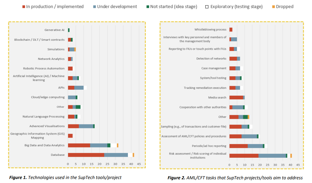
It’s evident from Figure 1 that current efforts focus primarily on improving data quality and scalability, essential foundations for effective SupTech. More advanced technologies like Generative AI, Blockchain, and network analytics are still in early stages but are expected to play a larger role in the future.

On the task side, presented in Figure 2, most tools are geared toward risk assessment, which appears to be the most straightforward application of SupTech. As the technology matures, other areas of AML/CFT supervision may benefit from more advanced capabilities as well.

Advantages and challenges

The EBA’s survey revealed several benefits from current SupTech initiatives, with most projects targeting improvements in data quality, analytics, adaptability, automation, and collaboration through standardization. SupTech enables supervisors to operate more efficiently, respond faster to emerging risks, and make better-informed decisions in a complex financial landscape.

However, fully embracing a data-driven approach comes with challenges. SupTech tools rely heavily on robust IT infrastructure, skilled personnel, and high-quality data. While these tools can help improve data quality by detecting anomalies, they still require reliable input to function effectively.

Legal risks also emerge, particularly around GDPR compliance and accountability for decisions made by opaque algorithmic models. Resistance to adoption may arise due to concerns about job displacement and trust in AI. Additionally, limited collaboration between institutions can lead to duplicated efforts and inefficiencies. Fortunately, the new AML/CFT framework offers a foundation for improved cooperation and information sharing across borders.

How can banks prepare for a successful transition?

Although the EBA’s report is aimed at supervisory authorities, it has important consequences for banks, payment providers, and other obliged entities. SupTech will help supervisors operate more efficiently and gain deeper insights, but it will also raise expectations for the institutions they oversee. Banks should prepare for increased data requirements, more rigorous scrutiny, and pressure to standardize and respond quickly to regulatory changes. While these requirements may pose short-term challenges, they will ultimately support better compliance, risk management, and operational resilience in the long run. In order to get there, Zanders supports institutions in key areas:

1. Increased data demands: AI-driven tools allow supervisors to process and analyze more data, requiring institutions to provide cleaner, more structured datasets.
2. Increased detail orientation: SupTech tools detect anomalies and patterns faster, meaning institutions must ensure accuracy and consistency in their reporting.
3. Standardisation:  EU-wide platforms and data-sharing standards will require institutions to align systems and formats for seamless supervision.
4. Change management: For SupTech to be successfully implemented, organizations must actively build a digital-first culture and encourage staff to move away from existing processes and mindsets.
5. Rapid adaptation: As technology evolves, supervisors will expect institutions to keep pace. Falling behind could lead to compliance gaps.

These challenges require strategic attention and tailored support. 

Are you interested in how Zanders can guide your organization through this transition? Reach out to our Partner Sebastian Marban.

As the European Union increasingly emphasizes robust digital resilience within the financial sector as of January 17^th 2025, the Digital Operational Resilience Act (DORA) has become a critical benchmark for compliance. A recent survey conducted with 23 banks reveals insightful data on their preparedness across various DORA categories. This blog dives into the findings and assess how well banks are positioned in meeting these regulatory standards. 

General Requirements: Solid Foundations, Communication Gaps 

The survey indicates strong compliance with foundational DORA requirements. Almost all banks have designated management functions for digital operational resilience and documented strategies. However, notable gaps exist in communicating these strategies effectively—as highlighted by the sizable number of banks without comprehensive stakeholder communication plans (12 “yes” vs. 11 “no” responses). Additionally, less than half the respondents have formal ICT risk appetite statements approved by senior management, leaving potential gaps in aligning risk management with organizational tolerance levels. 

ICT Risk Management: Comprehensive Yet Evolving 

Banks demonstrate proficiency in risk management frameworks with most having formal processes for risk identification and documentation. However, only about half systematically manage emerging and innovative technology risks—a critical aspect in today's evolving digital landscape. Equally concerning is the relative lack of focus on interconnectedness and concentration risks, with only 12 banks integrating these considerations into their risk assessments. 

ICT Resilience Testing: Gap Between Basic and Advanced Practices 

While regular ICT resilience testing is generally practiced, the adoption of advanced testing methodologies, such as threat-led penetration testing, is limited among the institutes that are required to perform these tests. Variability also exists in the processes for escalating issues and validating results, signifying areas requiring further attention. 

ICT Third-Party Risk Management: Variable Partnerships Management  

The survey reveals that while vigilance exists in maintaining third-party risk management frameworks, there are significant concerns regarding the strength of contractual safeguards and incident management processes. Less than half the banks have robust exit strategies or cater to geopolitical risks—a critical oversight in managing potential external disruptions. 

Incident Reporting: Strong Foundations with Room for Procedural Enhancement 

The incident reporting results indicate well-established bases in documentation and reporting processes. However, training in incident reporting procedures remains less uniform, which could impact consistency in handling real incidents. 

Business Continuity and Disaster Recovery: Recurring Gaps in Comprehensive Coverage 

While the majority of banks report having BCDRPs in place, only 16 ensure comprehensive coverage of all critical business functions. Testing and updating these plans is similarly underwhelming, staying mostly stagnant, which could hinder timely recovery efforts in case of an outage. 

IT-Security: Solid Security Postures with Continuous Improvement Needed 

Encouragingly, all respondents have documented ICT security policies, and most banks have appropriate security controls in place. While programs for regular updates in policies and controls are broadly adhered to, continuous improvement through employee training and periodic evaluations of security measures remains essential. 

Beyond the Checklist: Embedding True Resilience into Operations 

This survey highlights that while the foundations for DORA compliance are well-established within the banking sector, several areas still require strategic enhancements. Bridging communication gaps, enhancing advanced testing, improving third-party engagements, and boosting procedural training will be key to transitioning from foundational compliance to comprehensive resilience. 

These study insights serve to underscore not only the importance of regulatory adherence but also the critical need for continuous evaluation and proactive adaptation of digital resilience strategies amidst ever-evolving digital challenges. As banks continue this journey, the collective focus should remain on creating a more adaptive, secure, and resilient digital future. 

To find out more about DORA compliance and meeting regulatory standards, please contact our partner Martin Ruf.   

Managing banking book risk remains a critical challenge in today’s financial markets and regulatory environment. There are many strategic decisions to be made and banks are having trouble applying homogeneous hedging approaches across their balance sheet. As shown in the EBA’s IRRBB implementation heatmap of last February, hedging strategies and NMD modeling practices still vary significantly between banks. In addition, the EBA expects future developments on CSRBB and DRM. Meanwhile, behavioral risks and rapidly changing interest regimes need to be addressed, while balancing the stability of net interest income and economic value. 

Treasury departments are at the heart of managing the banking book, with their ‘ALM framework’ serving as the essential blueprint for banking book management. This framework ensures alignment between risk appetite and business objectives. A well-developed ALM framework provides better insights and enhances understanding of the balance between risk and performance.  

But, what are the characteristics of a mature ALM framework? What steps can be taken to elevate the maturity of the framework? And how can your framework unlock your full potential? This article explores the components that make up an effective ALM framework and describes what an advanced setup looks like. After inspecting ALM governance, risk frameworks, hedging strategies, ALM modeling and capital & performance management, we offer the opportunity to benchmark the maturity of your own framework against other banks and the ideal setup by filling out this survey. 

Governance 

The cornerstone of any effective ALM framework is appropriate governance, much like any well-functioning business activity. Setting up strong governance begins with defining a charter with a clear scope and mandate for the departments involved. It is crucial that the first and second line of defense have accurately defined roles and pro-active knowledge sharing needs to be the standard. Oversight by senior management is essential across all activities within the framework and the Asset-Liability Committee (ALCO) should be composed of members from treasury, risk and the business. 

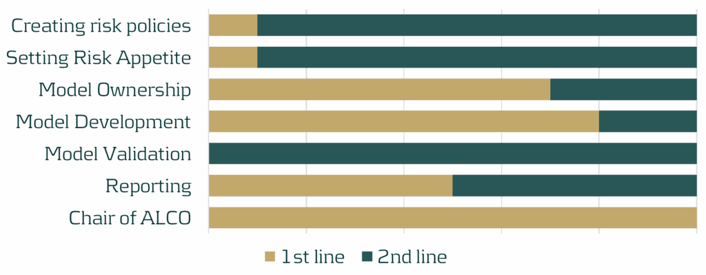
Figure 1: Distribution of roles and responsibilities of the first and second line, based on a survey performed by Zanders. 

Another critical element of ALM governance is the ALM strategy and the associated policies. The ALM strategy covers how risk and return are balanced, what interest rate position is ideal and how risks are operationally hedged (granularity, frequency and instruments). Typically, banks operate most effectively when the strategy is owned by the treasury department. The strategy should integrate perspectives on interest rate risk, credit spread risk, (intraday) liquidity risk, FX risk and capital, and must be fully aligned with business objectives and overall risk appetite.  

The second line should manage the translation of the strategy into comprehensive risk policies covering the same risk types and ensuring alignment with both global and local regulatory frameworks. As part of the overarching policy framework, a risk identification process must highlight emerging risk and feed into the Risk Appetite Setting (RAS). In turn, the RAS needs to define KPIs for guiding daily risk management, specifying the boundaries within which the first line can balance risk and return. 

Risk Framework 

Beyond sound governance, risk policies are integral to the broader risk framework. Within this framework, it is crucial to make informed decisions on measuring and hedging each individual risk type. Ideally, all risk types are managed within a central ALM system that supports risk dashboarding and stress testing. 

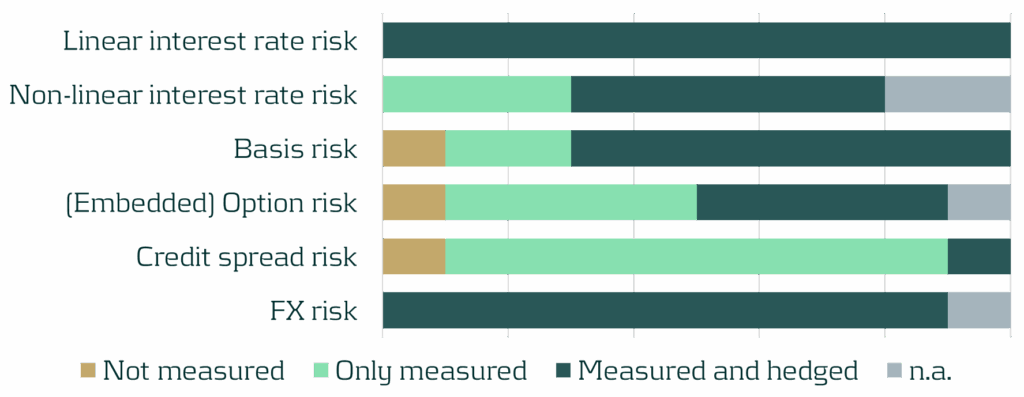
Figure 2: Risk- scope for a selection of sub-risk types, based on a survey performed by Zanders. 

In addition to identifying relevant risks and determining appropriate responses, it is essential to establish an internal operational framework for ongoing management. Centralizing and netting risks in central treasury books is fundamental to an efficient treasury function. While several approaches exist, internal transactions are typically preferred, as they enable accurate measurement of risks over different commercial and/or geographical portfolios. 

The strategy for managing interest rate risk in the banking book should ultimately be reflected in a clearly defined target duration of equity. Segregating the structural position into a dedicated book facilitates precise monitoring and agile adjustments to market dynamics and regulatory changes. Market volatility may necessitate revisiting the target based on interest rate expectations, and many banks have been adjusting their target durations accordingly. The structural position is a critical strategic choice in the trade-off between earnings and value stability, and is thereby an essential factor in the hedge strategy. 

Hedge Strategy 

With the risk framework, the treasury strategy, and risk appetite statement as its foundation, a strategy for hedging must be defined. This strategy guides first line processes, stating clear objectives on both earnings and value stability. Striking a balance between these two elements is challenging, but forms the basis for optimizing the balance sheet. The decision to include or exclude margins should be consistent across cashflows and discounting and should be aligned with the primary hedging focus, whether it is stabilizing earnings or value. 

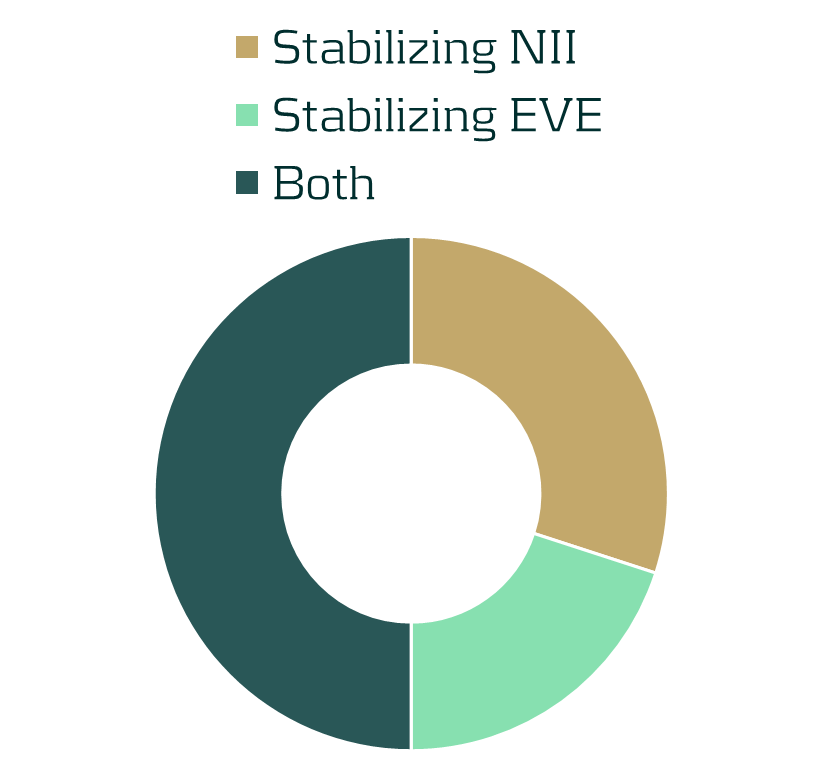
Figure 3: Focus of hedging strategies, based on a survey performed by Zanders. 

The scope of the hedging strategy must be consistent with the risk scope outlined in the risk framework and encompass the entire balance sheet. The strategy needs to address linear risks, and also explicitly account for non-linear risks that may arise due to convexity or behavioral factors.  

While commercial books typically have the objective to stabilize or increase net margins without taking an active position, hedging must be an active steering process. The treasury function should focus on optimizing the economic value of equity and net interest income within defined target limits. It is essential for the hedging process to be dynamic, using real-time analytics to proactively identify opportunities for improvement as market conditions and expectations change. Banks need to make use of scenario planning and predictive modeling to anticipate hedge requirements and adapt accordingly. 

Modeling 

Hedging practices are based on the outcomes of a bank’s models, which should reflect reality as close as possible. A challenging yet essential aspect to modeling is addressing the optionalities inherent to many financial products. These embedded optionalities need to be modeled consistently for all assets and all liabilities. Ideally, banks have advanced interest rate-dependent behavioral models in place to model the interest rate sensitivity of deposits and loans. Pipeline risk, the migration between different deposit types and potential other behavioral characteristics of products also need to be modelled. These models provide banks with realistic insights into expected cashflows. As customer behavior can vary significantly under different market conditions, banks benefit greatly from simulating and analyzing these changes using stochastic models. 

Figure 4: Type of behavioral modeling performed by banks, based on a survey performed by Zanders. 

From a liquidity perspective, it is important for banks to use consistent methodologies for short and long-term cashflow forecasting. Additionally, integrating liquidity models, such as those for LCR and NSFR, with liquidity stress testing, offers valuable insights into potential future liquidity needs. 

Machine learning is gaining more and more traction within the field of ALM and is becoming an integral part of ALM modeling. Using machine learning for client segmentation is increasingly more common and helps in better understanding client behavior. Several machine learning techniques for (reverse) stress testing have been developed, which improve the ability to identify vulnerabilities in balance sheets. Furthermore, predictive analytics helps to optimize balance sheet management, empowering banks to make informed strategic decisions.

Capital and Performance 

Final critical elements of strategically steering a bank are the management of capital and performance measurement. Capital management is a fundamental part of modern-day banking and one of the important factors in balance sheet management. Mishandling capital requirements can significantly impact competitiveness and distort the view of risk-adjusted performance. To manage capital effectively, banks need to identify the ex-ante cost of capital for each transaction and incorporate it into pricing. Capital requirements should be allocated at the transaction level, allowing for accurate calculation of capital usage per portfolio. Ongoing capital monitoring and alignment to stress testing exercises and risk appetite is essential for optimal capital allocation and planning. 

An effective Funds Transfer Pricing (FTP) framework is essential to assess risk-adjusted performance at the transaction level and to allocate overall performance across business units. In a mature FTP framework, all products are priced using an internally determined FTP curve. At a minimum, this curve needs to reflect the interest rate and liquidity risks inherent to transactions, but it can be extended to incorporate other types of risk. The FTP curve must be dynamic, adapting to portfolios and market conditions. Moreover, the FTP curve should be governed by senior management, who adjust it as needed to steer the balance sheet through (dis)incentivizing specific products or maturities. 

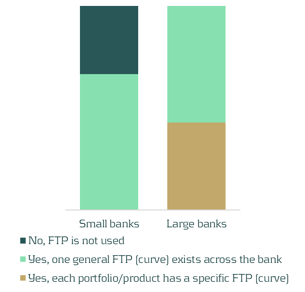
Figure 5: Usage and granularity of FTP frameworks, based on a survey performed by Zanders. 

Conclusion 

The key to successfully managing banking book risks is an effective ALM framework. By leveraging your ALM framework and ensuring it aligns with the bank’s overall strategy, business objectives and complexity, you can enhance treasury’s performance and effectively manage the increased regulatory attention to IRRBB strategies. 

At Zanders, we developed a model to assess the maturity level of a bank’s ALM framework. The model provides valuable insights into the maturity of the individual components and the ALM framework as a whole. This facilitates quick and straightforward benchmarking. 

We invite you to complete the survey below and participate in the benchmarking exercise, which should take you less than 10 minutes. We will analyze your answers and share the (anonymized) findings with you. 

ALM framework benchmarking survey 

Please contact Erik Vijlbrief or Jelle Thijssen for more information. 

On July 2nd, the European Banking Authority (EBA) published a Consultation Paper proposing amendments to its 2016 Guidelines on the application of the definition of default (DoD). As part of the consultation process, open until 15 October 2025, the credit risk specialists at Zanders will submit a formal response, leveraging our extensive experience in DoD regulation and implementation.

In this article, we share our perspective on three of the EBA’s proposed amendments, focusing on the potential impact and implementation challenges for institutions:

• We expect that a shorter probation period for forbearance measures (that only alter the repayment schedule leading to a NPV loss not greater than 5%) are expected to provide incentives for banks to opt for those types of measures rather than the most sustainable ones.

• We recommend the EBA to implement EU wide DoD guidelines they considered for payment moratoria (similar to the one for Covid), whereas the EBA proposes not to. Zanders would approve permanent moratoria guidelines, as it clarifies if governmental moratoria introduced for climate risk related natural disasters should be regarded as forbearance.

• We are oncerned that the proposal to consider material arrears on non-recourse factoring exposures up to 90 (instead of 30) DPD as technical past due situations could result in an undesired increase in the percentage of IFRS stage 1 exposures migrating directly to stage 3 (impairment).

The following chapters elaborate on these three proposed amendments in more detail.

Forbearance

The first amendments addressed in the EBA’s consultation paper (CP) are related to forbearance. The supervisory authority explains that an increase of 1% threshold for a diminished financial obligation (DFO) to 5% was considered for certain forbearance measures. This follows from the European Commission’s mandate that the update of the EBA guidelines on DoD“… shall take due account of the necessity to encourage institutions to engage in proactive, preventive and meaningful debt restructuring to support obligors.”¹

In the EBA’s current DoD guidelines (DoD GL), a forbearance measure leading to a 1% or more DFO results in a default classification, which could discourage institutions from applying these measures. However, the CP purposefully proposes to exclude an increase to a 5% DFO threshold, since institutions can already implement strict(er) forbearance definitions (i.e. for concession, financial difficulty) to prevent undue default classifications. Instead, the EBA proposes to shorten the probation period from 12 to 3 months for forbearance measures that: (1) only lead to suspensions or postponements and not e.g. changes to the interest rate or exposure amounts and (2) leading to less than 5% DFO loss.

This treatment will likely incentivize institutions to choose forbearance measures in scope of the shorter probation period, rather than the ones that would be optimal for a “sustainable performing repayment status” of the obligor. The latter would be in line with the EBA’s own requirements on the management of forborne exposures (Par. 125 EBA/GL/2018/06). Furthermore, the fact that the EBA does not set the “predefined limited period of time” for the measures in scope could lead to RWA variability, as some institutions may apply the shorter probation period to longer duration forbearance measures than others. For example, if Bank A sets the limited period of time to 6 months, they can apply the shorter probation period more often compared to Bank B, which sets the period of time at 3 months. Finally, it appears as if the proposal of the banking authority aims at favouring granting forbearance measures in scope to obligors with short-term (rather than structural) financial difficulties. That is, the EBA explains that the forbearance measures in scope of the shorter probation period treatment “… would most likely be viable for obligors in temporary financial difficulties”. The shorter probation period would then lead to a return to a performing status earlier for obligors to which the forbearance measures in scope are extended, which leads to a better RWA for these obligors. Alternatively, a distinct probation period (or even higher DFO threshold) could be proposed for obligors in short-term financial difficulties, as defined in Paragraph 129(A) of the EBA’s guidelines on Management of Forborne Exposures. This would also achieve the EBA’s goal, without influencing institutions’ decision about which forbearance measure to apply.

It should be mentioned that while a large RWA impact is not anticipated from the establishment of a distinct probation period, there will likely be a significant implementation burden associated with the change. This is because, as multiple forbearance measures are usually adopted in tandem, different probation periods must be traced concurrently. The implementation of this modification would need to be retroactive, though, as credit risk models will need to be recalculated using adjusted historical data in order to account for this change. In the past, retroactively modifying the probationary period has proven to be a time-consuming and expensive problem.

Legislative payment moratoria

In light of the COVID-19 crisis, the EBA published guidelines in 2020 on handling payment moratoria introduced by governments as a means of financial aid in the context of forbearance. For certain COVID-19 measures allowing e.g. a grace period in scope of the guidelines, EBA/GL/2020/02 and amendments in .../08 and …/15, would not in itself require institutions to classify the exposures as forborne.

Even though the EBA considered introducing guidelines for potential future moratoria, the CP proposes against these changes. As one of the arguments against new moratoria guidelines, the EBA remarks that moratoria in itself will not result in DFO loss of more than 1%, hence not leading to defaults. The EBA implies that introducing new moratoria guidelines would therefore be obsolete. The EBA is also worried about RWA variability that might arise if governments declare legislative moratoria for crises in their jurisdictions. That is, the EBA expects that intra-EU comparability of RWA across institutions, might be compromised.

Adding the considered guidelines describing when moratoria should lead to forbearance in the amended DoD GL is advisable, even though the EBA proposes in the CP to remove them. Zanders challenges that guidelines describing when moratoria do not lead to forbearance would not be necessary, because the 1% DFO threshold will not be met. That is, Zanders highlights moratoria guidelines would still decide when the forborne status should be assigned to exposures if moratoria are applied. This forborne status impacts the default status later on, both for performing and defaulted exposures. The reason is that if performing forborne exposures become 30 days past due within 24 months after receiving the forborne status, a defaulted status should be assigned. If the moratoria do not lead to a forborne status, these exposures should default after becoming 90 days past due on a material amount instead. Furthermore, for defaulted exposures, it is important to understand when moratoria result in the forborne status and when they do not. That is, in order for a forborne defaulted exposure to go out of default, a substantial payment and an extended cure period are needed. Zanders would therefore be in favor of EBA guidelines that specify when moratoria should result in a forborne status and when this is not necessary.

As for the RWA variability, as self-identified by the EBA, stringent criteria could be introduced prescribing what moratoria are in scope of the amended DoD GL. As described by the EBA as well, in light of climate risk related natural disasters, payment moratoria could occur more often as a governmental means of financial aid. In contrast to ad hoc rules for each specific crisis, such as observed during the COVID-19 pandemic, Zanders contends that permanently applicable moratoria instructions in the updated DoD GL will eventually lead to a more stable RWA impact when economic or natural catastrophes occur.

Days past due for non-recourse factoring

Paragraph 23(D) of the current version of the DoD guideline stipulates that in the specific situation of non-recourse factoring for which the arrears materiality threshold is breached, but none of the receivables is more than 30 days past due (DPD), should be treated as a technical past due situation. Non-recourse factoring refers to the situation where the institution (e.g. a bank) has bought receivables from its client (e.g. service provider) owed by the debtor (e.g. service consumer). The idea behind the 30 DPD is that the DPD counter might continue to increase due to a consecutive overlap in non-payments of invoices, lengthy administrative processes, and a low degree of control of the institution over the invoices.

The CP proposes to allow for up to 90 DPD to be considered technical past due situations, in correspondence to the industry requesting the EBA to be more lenient in the DoD guidelines for non-recourse factoring. This is motivated by the fact that many corporates have at least one invoice past due more than 30 days, while being rated investment grade.

Although Zanders understands  corporates’ need for more leniency, allowing for up to 90 DPD to be recognized as technical past due could make stage 2 obsolete for IFRS provisioning models. That is, if material arrears on non-recourse factoring exposures should be considered technical past due for situations up to 90 DPD, the said exposures will move from 0 DPD to 91 DPD in one day. The additional lenience would break the desired flow of exposures transitioning from IFRS stage 1 (performing), first towards stage 2 (significant increase in credit risk), before going to stage 3 (credit impaired). This stage migration effect could be mitigated by another stage 2 trigger: forbearance. However, the institution cannot apply forbearance measures to a sold invoice that is due to the institution’s client, rather than due to the institution itself. Therefore, as a stage 2 trigger, forbearance cannot compensate for the lack of the30 DPD in the particular scenario of non-recourse factoring risks.

Zanders proposes to find a balance between leniency on DoD guidelines and stage migrations, by increasing the 30 days threshold. The proposed number of days should be based on an analysis of non-recourse factoring portfolios from a representative sample of supervised institutions. This analysis should then strike a balance between the average observed days past due of invoices sold on the one hand and the representativeness of IFRS stage transitions on the other hand. Zanders is convinced that amending DoD GL based on this analysis will prevent the undesired impact on IFRS provisioning models and will better fit European corporate invoicing practice.

Conclusion

In this post we analysed 3 proposed amendments from the published Consultation Paper, in which the European Banking Authority (EBA) proposes amendments to its 2016 Guidelines on the application of the definition of default (DoD).  Alternatives are suggested for all 3 proposed amendments as the proposed amendments leave room for improvements .

Reach out to our experts John de Kroon and Dick de Heus, if you are interested in getting a better understanding of what the proposed amendments mean for your credit risk portfolio.

We monitor the progress of the Consultation Paper in the future. Keep a close eye on our LinkedIn and website for more information, or subscribe to our newsletters here.

Artificial intelligence (AI) is advancing rapidly, particularly with the emergence of large language models (LLMs) such as Generative Pre-trained Transformers (GPTs). Yet, in quantitative risk management, the perceived utility of these technologies remains relatively narrow. Most current applications focus on technical use cases, such as code autocompletion within Integrated Development Environments (IDEs), to boost productivity for developers and quantitative analysts. While valuable, these uses only hint at AI’s broader potential. Limiting AI to technically knowledgeable users overlooks opportunities to empower a wider range of stakeholders, including those without programming skills. 

In this article, we explore AI agent frameworks, highlight their potential to enhance various banking functions, and share our thoughts on key design considerations when using agents in risk-sensitive environments. 

What exactly are AI agents?

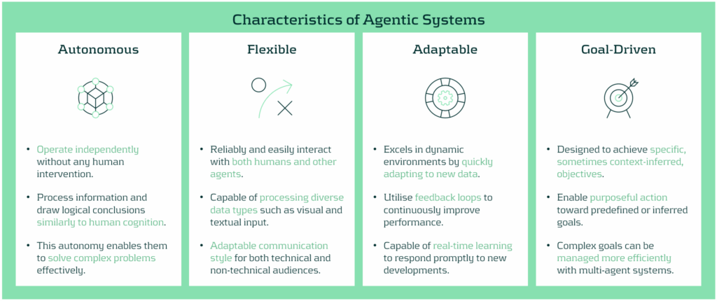
While the definition of an AI agent may vary depending on the specific use case, they are generally characterised by a high degree of autonomy and a goal-oriented design. A recurring theme in the development of these systems is their ability to operate independently across entire analytical workflows. This marks a shift in how AI is utilised - transforming models from passive tools or advanced search engines into active, decision-making agents capable of driving end-to-end processes. 

In the context of risk management, these workflows might include executing models, validating outputs, conducting ongoing monitoring and review, running sensitivity analyses or stress tests, and generating model performance reports. Interestingly, these actions can all be initiated by a simple trigger, often in the form of a natural language prompt - a method that has become increasingly familiar. Unlike conventional systems designed for single tasks, agents are built to reason, decide, and act across multiple steps, adapting to requirements with flexibility. 

A typical agent architecture consists of five core components: 

1- Interface Layer / Trigger: Translates business-level questions (e.g., “What’s the impact of a 25% increase of default probability on risk-weighted assets?”) into executable workflows, enabling non-technical users to trigger complex analyses. 

2- Input and Data Processing: Preprocesses and transforms input data or outputs from other checkpoints into structured data that can be used in the agent’s decision-making process.  

3- Memory & Context Manager: Maintains a record of prior steps, decisions, and user inputs to guide multi-stage processes intelligently and retain context over series of interactions. 

4- Tool Integrator: Connects to and uses various tools (such as Python environments, databases, APIs, and model libraries) to perform technical tasks. The agent dynamically works out which tool is relevant for executing specific tasks based on predefined instructions. 

5- Large Language Model (LLM): Determines the sequence of actions needed to achieve a specific goal, e.g. “Backtest this IRB model under a recession scenario”. In this example, the LLM would identify actual periods spanning a receding economy and uses the corresponding data to execute the model and return the results. 

This architecture allows AI agents to operate like digital collaborators, fetching and processing data, visualising results, and helping to explain patterns that we may otherwise miss - all without requiring users to interact with a single line of code. 

Benefits of AI Agents Across Different Banking Functions 

Beyond improving information access, AI agents deliver strategic benefits through automation, broader access to analytical tools, faster decision-making, and the removal of process bottlenecks. Here’s how agentic solutions support various stakeholders: 

• Front Office (Trading, Structuring, Portfolio Management): Enhance front-office functions including pre-trade analysis, data acquisition and processing, continuous market monitoring, and rapid trade execution. By integrating structured and unstructured data, ranging from market sentiment to fundamental and technical indicators, the agents allow trading and investment professionals to make faster, more informed decisions that are grounded in a holistic view of market conditions. 

• Risk Modeling and Analytics Teams: Aid modelers to accelerate prototyping and calibration by offloading repetitive tasks such as parameter sweeps, benchmarking, or sensitivity runs. Agents can also assist with documentation and help iterate on design logic more efficiently, freeing up time for more complex problem solving. 

• Model Risk Management (MRM): Streamline model validation through automation and a system designed to enhance efficiency and reliability. The system can independently replicate results from model execution, generate challenger models, and document testing steps, offering a transparent and auditable workflow that strengthens governance and reduces approval timelines. 

• Risk Control and Regulatory Reporting:  Automate aspects of stress testing and capital reporting for control functions. By having the ability to recalculate model results under different model assumptions, maintaining traceable logic, and generating consistent documentation, the agents help ensure model results align with regulatory standards. 

Ensuring Trust and Quality with AI Agent Solutions: Oversight, Governance, and Guardrails 

As promising as AI agents are, their deployment in risk-sensitive environments must be accompanied by robust controls. Key design considerations include: 

• Security: Solutions are restricted to rely only on credible and approved AI models or models that have demonstrated high safety for institutional use. All other components are designed in Python, eliminating risks that may be posed from third-party systems and processes.  

• Data Governance: Agents only access approved, secure data sources, with permissions and version control strictly enforced. Where privacy is critical, data anonymisation or summarisation techniques can be applied. 

• Explainability: Transparency is ensured through well-defined workflows, step-by-step process documentation, and audit trails to help stakeholders understand how decisions are made. 

• Scope Boundaries: Agents operate within clearly defined limits (e.g., executing but not creating new models). A human-in-the-loop approach is used for material-risk decisions, while lower-risk processes may be fully autonomous. 

• Validation: Like any model, agents undergo rigorous testing for accuracy, consistency, and robustness, especially in edge cases. By applying the traditional “three lines of defense” model to AI agents, oversight and accountability is embedded into their lifecycle. 

Conclusion 

AI agents offer enormous potential to drive automation and expand access to analytical tools, especially for non-technical stakeholders. This facilitates deeper integration of business and regulatory expertise into processes across trading, reporting, and model development. When built with strong governance, robust data controls, and transparent logic, AI agents don’t just support critical workflows, they improve them. 

At Zanders, we support clients in understanding how AI agents can benefit their risk management frameworks to unlock operational efficiency and expand access to advanced analytics. For more information on how Zanders can help you to utilize the power of AI agents, contact Dilbagh Kalsi (Partner) or  Stanley Nwanekezie (Manager). 

In an industry where growth is often measured in multiples, and value creation is expected to be both scalable and repeatable, operational excellence is no longer a supporting function—it’s a strategic enabler. Yet one of the most fundamental enablers of value creation remains underdeveloped across many private equity-backed businesses: the financial value chain.

This system—spanning everything from working capital and liquidity to payments, banking, and treasury technology—often determines whether a company can scale without friction, execute M&A efficiently, or respond to volatility with speed. And at the heart of that system lies a single objective: cash agility.

Why Cash Agility Matters in PE

Private equity firms have long emphasized growth acceleration, M&A, and operational leverage as core value drivers. These remain powerful levers—but they are increasingly vulnerable to delays, integration challenges, and market-driven volatility. What’s less volatile, and arguably more repeatable, is a firm’s ability to control and redeploy its own capital faster.

Cash agility describes the capability to mobilize internal liquidity—whether to seize investment opportunities, fund strategic initiatives, or manage downside risks—without unnecessary friction or reliance on external capital. It represents the intersection of visibility, control, and speed across the financial value chain.

In this sense, cash agility is about creating an institutional capability to convert operational execution into strategic flexibility.

The Financial Value Chain: A Missed Opportunity

In many portfolio companies, the financial value chain is fragmented. Processes have evolved piecemeal, often in response to tactical needs rather than strategic planning. Treasury sits apart from commercial functions. Working capital is optimized through isolated projects. Systems don’t talk to each other. Spreadsheets fill the gaps between data, decision, and executionAs a result, CFOs and PE sponsors alike struggle with basic questions:

How much cash is available across the group today? Where is it trapped? Can it be upstreamed, invested, or deployed without delay?

In our recent project with a mid-market portfolio company, the finance team had to manually consolidate bank balances from over 200 accounts across 30 entities to produce a weekly liquidity report—consuming hours of effort and often resulting in outdated insight. The company had been growing fast through M&A, but its cash visibility had not kept pace. This created real constraints when the group needed to move quickly on a bolt-on acquisition, forcing reliance on external bridge financing and delaying execution by weeks.

This scenario is common across mid-sized and even large PE-backed businesses. And while every firm understands the importance of “cash control,” few have turned that awareness into a repeatable capability.

From Fragmentation to Agility: What Good Looks Like

Building cash agility starts with aligning the components of the financial value chain into a cohesive, strategically designed operating model. This typically includes:

• Real-time cash visibility across all entities and currencies, ideally enabled through TMS/ERP integration and automated bank feeds.
• Forecasting processes linked to operational and commercial drivers, integrated with actual cash positions—offering a forward-looking, actionable view of liquidity rather than a static snapshot.
• Banking architecture designed for mobility over rigidity—supporting automated sweeps, intercompany lending, and minimal account fragmentation.
• Payment processes embedded with control but freed from manual bottlenecks—using centralized workflows, audit trails, and fraud prevention tools.
• Capex and working capital governance that prioritizes ROI, liquidity impact, and execution timing over pure budget conformance.
• Cash flow management as a continuous fitness program for liquidity—driving productivity, improving free cash flow, and delivering more sustainable performance than reactive working capital initiatives alone.

For PE investors, the ultimate test of these systems isn’t operational elegance. It’s whether they enable faster execution, more efficient capital deployment, and consistent delivery of the investment thesis.

Common Bottlenecks

Across Zanders’ private equity engagements, several recurring issues tend to slow progress toward cash agility:

• M&A Complexity: Acquisitions bring in diverse systems, bank setups, and control environments. Without a clear treasury integration playbook, complexity compounds.

• Underinvestment in Treasury: Many companies have no dedicated treasury function or treat it as a back-office necessity despite a highly positive business case. This leads to disjointed tools, lack of ownership, and reactive problem solving.

• Disconnected Systems: ERP, TMS, and bank portals often operate in isolation. Without an integrated architecture, data is delayed, duplicated, or distorted.

• Legacy Banking Landscapes: Companies often maintain outdated banking setups, including hundreds of rarely used accounts or manual payment processes that create risk and inefficiency.

• Static Forecasting: Forecasts are built manually, reviewed infrequently, and rarely integrated into daily cash decisions.

Solving these challenges requires more than a few process tweaks. It demands a step change in how financial operations are conceived, designed, and executed.

Case in Point: When Financial Architecture Drives Value

In one engagement with a global consumer technology leader generating over $40 billion in annual revenue, Zanders helped transform an inherited web of disconnected financial operations into a single, scalable treasury architecture. The company had expanded rapidly, but its cash remained fragmented across geographies and systems. We centralized liquidity into a unified control structure, redesigned the firm’s bank strategy and FX risk setup, and implemented automated cash processes through an in-house bank.

The results were transformational. Annual costs dropped by $18 million, and over $8 billion in trapped cash was unlocked for reinvestment. Treasury operations became leaner, with over $10 million in savings achieved through rationalized account structures and reduced IT system costs. Perhaps more strategically, the business freed up $17 to $35 million in withheld taxes by migrating treasury entities—capital it could now allocate to growth, innovation, or debt reduction. What had once been an operational bottleneck became a value multiplier.

Another engagement with a multinational education group revealed the power of standardization at scale. With 80+ campuses across continents and multiple ERP systems, treasury processes were fragmented and reactive. Zanders introduced a centralized target operating model, implemented a TMS integrated with the group’s ERP infrastructure, and deployed straight-through-processing to streamline reporting and control.

As a result, the company now saves $3.8 million annually, has released $1.7 million in working capital, and accumulated a projected $14 million benefit over a five-year horizon. More importantly, it has increased cash forecasting accuracy, reduced manual workload, and enhanced operational resilience—capabilities that will serve the group across future growth cycles.

Cash Agility: A Lever for Repeatability

For private equity investors, the question isn’t whether cash agility creates value. It’s whether it creates value that’s consistent, transferable, and visible to the next buyer.

Too often, value creation initiatives focus on EBITDA expansion—growth, margin improvement, pricing, procurement. These levers are critical, but they are also cyclical, competitive, and often constrained by talent or timing.

The financial value chain offers a different type of leverage. When optimized, it unlocks value that is self-funding, recurring, and resilient. Cash agility enhances decision velocity, reduces the cost of capital, and minimizes execution risk. It also makes businesses more attractive at exit by demonstrating financial discipline, liquidity control, financial risk awareness and systems maturity.

This is especially relevant in today’s environment, where LPs and acquirers scrutinize not just the numbers, but the operating backbone behind them. Clean books and good margins are important—but increasingly, buyers want to know: Can this company manage growth? Can it scale its financial systems? Can it fund itself efficiently?

These are questions cash agility helps answer.

Where Zanders Fits In

Zanders works with both PE sponsors and portfolio companies to build this capability. Our role is to serve as an external financial operating partner—focused on aligning finance execution with investment priorities.

We combine strategic thinking with hands-on implementation, delivering projects that range from working capital diagnostics to full treasury transformations. Our clients include global PE houses, mid-market sponsors, and management teams navigating carve-outs, integrations, and digital finance initiatives.

What distinguishes our approach is the focus on outcome: measurable improvements in cash visibility, efficiency, and control—not just slideware or process maps. We work with the CFO, but we work for the investor.

Cash Agility as a Strategic Outcome

Ultimately, cash agility is not an end in itself. It’s the enabler that turns capital into capability.

It allows portfolio companies to reinvest faster, fund growth internally, and respond to uncertainty with confidence. It gives CFOs the tools they need to lead, not lag, in execution. And it helps investors translate operational improvements into multiples—by building the infrastructure of repeatability.

In a market where capital is no longer cheap, and execution risk is rising, agility is not a luxury. It’s a requirement.

With extreme weather events becoming more frequent and climate policy tightening across jurisdictions, banks are under increasing pressure to understand how climate change will impact their portfolios. Previously, most climate scenario analyses have focused on long-term trajectories, stretching out to 2050 or beyond. However, these long-term analyses have often been far too abstract for day-to-day risk management.

The new NGFS short-term scenarios investigate the impact of climate risks over the next five years, offering a more practical solution. By isolating the individual impacts from physical and transition risk, and by providing better granularity at both temporal and sectoral levels, the new scenarios provide a new and valuable tool for climate risk modeling.

In this article, we explore what makes these scenarios unique, their benefits and limitations, their impact on future macroeconomic and market trends, and importantly, how banks can utilize them to fulfil regulatory requirements.

Physical and transition risks in the scenarios

The short-term scenarios capture four possible futures, each reflecting a different mix of physical and transition risks. The scenarios show how varying levels of climate policy and climate-related events could shape the economic and financial outcomes over the next 5 years. The four scenarios are summarized in the figure below.

Figure 1: The four NGFS short-term scenarios.

Key benefits and limitations of the new scenarios

The scenarios offer several benefits, including a more practical time horizon and better isolation of physical and transition risks. However, they also come with inherent limitations that should be acknowledged when being used. Below, we summarise the main benefits and limitations of the new scenarios.

Benefits

• Time horizon
  • Although NGFS has already released several versions of their long-term scenarios, this is the first release of climate scenarios whose narratives focus on the next few years. Short-term scenarios cover time horizons that are typically more relevant for risk assessment management in banks, such as capital planning, liquidity assessments, and regulatory stress testing exercises. In addition, the uncertainty of climate and macroeconomic variables increase over longer horizons, making the short-term scenarios more dependable.

• Calibrated using recent data
  • As with any model which has been recalibrated using the latest data, by incorporating the most recent economic conditions, market trends, and climate policy commitments, the short-term scenarios provide more reliable and accurate forecasts. This allows banks to run more credible stress tests, develop informed strategies, and leads to outputs that are more aligned with current market and policy conditions.

• Isolation of physical and transition risk
  • Three of the four scenarios isolate only physical or transition risk, which can provide more targeted insights for climate risk assessment. By separating these risks, banks can identify the specific drivers of financial impact more accurately, whether from policy changes or climate-related events. Unlike scenarios that contain a combination of transition and physical risks, isolating only one of the risks can make the results easier to interpret and act upon.

• Variation across sectors and regions
  • NGFS short-term outputs cover up to 15 macro-regions (e.g. EU27, Asia and North America) and up to 46 countries, which is similar to the long-term scenario results. The biggest improvement is found on the temporal granularity: while most of the variables for the long-term scenarios are provided in 5-year intervals, the short-term scenarios are mostly provided on a yearly basis.

Limitations

• Still not short enough?

While the NGFS short-term scenarios aim to address near-term climate-related risks, even shorter time horizons may be necessary for accurate and practical modeling in both credit and, in particular, market risk. More granular timeframes, such as a quarterly projection interval, would support banks to rapidly react to policy changes, market reactions, or acute physical climate events, which can unfold within weeks or months and not years.

• Lack of dispersion within regions or sectors

In some cases, the results show limited differentiation between sectors and regions. This can make it difficult to accurately capture sector-specific or country-specific vulnerabilities. For example, countries with significant geographical and socioeconomic differences, such as Switzerland, Iceland, and Ukraine, are grouped together under the region "Rest of Europe". Similarly, the sector "Market Services" includes a wide range of distinct industries, such as Real Estate, Telecommunications, and Waste and Water Collection.

• Physical risk is still difficult to accurately model

Accurately capturing physical climate risk within a short-term horizon remains methodologically challenging. Acute events like floods or wildfires are based on the estimation of tail risks (e.g. return periods) which can be difficult to model accurately. In addition, physical risks exhibit high spatial variability. For instance, coastal areas can be more vulnerable to hurricanes than inland areas, even if they are in the same country. Therefore, aggregating scenario data on the country or regional level can potentially underestimate the risks in specific areas.

• Over-simplification of policy implementation

Policy pathways in the short-term scenarios tend to assume smooth, linear implementation and immediate effectiveness. In reality, climate policies often face political, social, and economic frictions that delay or prolong their impact. Hence, these assumptions may lead to the underestimation of transition shocks, particularly where abrupt or uncoordinated policy actions could trigger market volatility.

Impact of the new scenarios on important modeling variables  

To take a look at the NGFS short-term scenarios in action, we can examine the impact of the scenarios on key macroeconomic variables. Figure 2 shows the behavior of GDP and carbon price (with respect to baseline values) within Europe and Asia for all four scenarios. There are clear negative shocks which are seen in the GDP for all the scenarios. Similarly, we see a positive spike in the carbon price for both regions, however the effect in Asia is much greater than in Europe. Asia experiences a sharper percentage increase in carbon prices because it starts from a much lower baseline compared to Europe, where carbon prices are already high and policies have been in place for years. Additionally, in general, Asia is more emissions-intensive and heavily reliant on fossil fuels (particularly coal) which means more aggressive changes to carbon pricing are required to reduce emissions.

Figure 2: Top – YoY change in GDP (compared to baseline). Bottom – change in carbon price (compared to baseline).

Although the impact to variables such as macroeconomic indicators, emissions trends, and shifts in production offer essential context, they are usually only the first step in climate risk modeling. Ultimately, we are interested in how these variables translate into changes in market-based metrics, such as corporate bond spreads or PDs, which directly affect portfolio valuation. For example, for stress testing purposes, macro and sectoral outputs must be mapped onto these market-based metrics to assess potential losses and capital impacts.

Figure 3 compares the corporate bond spread adjustments for the Oil, EV Transport Equipment, and Hydroelectric sectors under the HWTP scenario. The results illustrate a shifting investor sentiment in the corporate bond market. The Oil sector experiences a significant increase in spread adjustments over the time horizon due to an increase in perceived risk and a decline in investor favorability. In contrast, the EV Transport Equipment and Hydroelectric sectors maintain negative spread adjustments, highlighting that they are viewed more favorably. Overall, these results capture a market preference for cleaner and more sustainable industries and the scenarios clearly distinguish between sectors that are carbon-intensive and those aligned with low-carbon technologies.

Figure 3: Adjustment to corporate bond spreads for the Oil, EV Transport Equipment, and Hydroelectric sectors (HWTP scenario).

Zanders’ opinion

Although the five-year horizon of the new scenarios is still somewhat too long for direct application to market risk modeling (where exposures fluctuate on much shorter timescales), it aligns far better with the lifecycle of most credit products, especially those with relatively short maturities such as personal loans. Banks should utilise the scenarios as starting points for modeling the effects of near-term climate shocks on the performance of their credit products. However, the new scenarios can still provide valuable insights for market risk modeling. The scenarios can help identify sectoral sensitivities, adjust volatility and correlation assumptions, and enrich the narratives of existing scenarios.

The scenarios also help to standardise climate stress testing by providing a consistent set of assumptions, variables, and modeling frameworks that financial institutions can use as a common reference. This alignment reduces discrepancies in inputs and methodologies, enabling more comparable results across banks and jurisdictions. As a result, institutions and supervisors can more effectively benchmark climate-related risks, identify outliers, and support coordinated regulatory responses, ultimately improving the credibility and usefulness of climate stress tests.

Importantly, the new scenarios are well-suited to meet the needs of regulatory frameworks like the Internal Capital Adequacy Assessment Process (ICAAP), which typically considers a 3-to-5-year horizon. This makes them far more applicable than traditional long-term scenarios, which typically look out to 2050. Similarly, the ECB climate stress testing framework requires banks to use a variety of time horizons and both physical and transition risk scenarios. With ever-growing regulatory expectations, such as the recent CP10/25 consultation paper from the PRA on managing climate-related risks, the new short-term scenarios provide a timely and relevant tool for banks.

Conclusion

The new NGFS short-term scenarios are an important addition to climate risk modeling frameworks, offering a direct focus on the next five years – a time period which is far more aligned with capital planning, liquidity assessments, and regulatory stress. However, the scenarios are not intended to replace existing long-term scenarios. Rather, they complement them by providing a near-term view of climate risk that is highly relevant for all banks.

For more information on how Zanders can support you to understand the impact of climate risk on your business, please contact Steyn Verhoeven and Polly Wong.

With the introduction of CRR3, effective from January 1, 2025, the ‘extra’ guarantee on Dutch mortgages – known as the Dutch National Mortgage Guarantee (NHG) – will no longer be automatically eligible for the modeling approach. This requires institutions to apply the substitution approach instead. Although this may seem like a minor change, it can have far-reaching consequences. In this article, we provide a background on this change in the treatment of NHG and discuss the potential implications and challenges it may bring. 

Introduction Dutch National Mortgage guarantee (NHG) 

The Dutch National Mortgage Guarantee (NHG) serves as a safety net for borrowers and lenders of mortgage loans in the Netherlands. It is designed to provide protection in cases of financial distress caused by circumstances such as divorce, disability, or unemployment ​[1]​​ [2]​​ [3]​. If these situations require the sale of the residential property and a residual debt remains after all other collection sources have been exhausted, the NHG will cover this remaining debt when contractual conditions are met¹. 

The NHG guarantee is provided by the Stichting Waarborgfonds Eigen Woning (WEW)​ [1]​​ [4]​. Although Stichting WEW is not state-owned, the Dutch state acts as a suretyship provider. This arrangement ensures that if Stichting WEW’s capital is insufficient to meet its guarantee claims, the state will supply unlimited interest-free loans. These loans must be repaid only after the foundation’s assets have been restored ​[5]​. 

Following the Capital Requirements Regulation (CRR), the NHG guarantee classifies as Unfunded Credit Protection (UFCP) Credit Risk Mitigation (CRM) and should be treated accordingly. 

Exposure class of Stichting WEW 

As outlined in the previous text, the direct protection provider of the NHG is Stichting WEW. In the event that NHG fails to make payments, the Dutch sovereign state provides a suretyship to Stichting WEW, essentially serving as a counter-guarantee for the NHG guarantee extended by Stichting WEW.  

CRR III article 4(8) ​[6]​ defines a public sector entity (PSE) as: “a non-commercial administrative body responsible to central governments, regional governments or local authorities, or to authorities that exercise the same responsibilities as regional governments and local authorities, or a non-commercial undertaking that is owned by or set up and sponsored by central governments, regional governments or local authorities, and that has explicit guarantee arrangements, and may include self-administered bodies governed by law that are under public supervision;”  

Stichting WEW satisfies the definition of PSE in CRR III article 4(8), as it is a non-commercial undertaking (stichting) established² by the central government, with an explicit guarantee arrangement from the Dutch central government. However, the CRR does not clearly define the sponsoring of the central government. Should it be determined that the sponsoring requirement is not met, Stichting WEW must instead be classified as a corporate exposure class³.  

The remainder of the text assumes that Stichting WEW can be classified under the PSE exposure class as defined in CRR III article 112(c) (SA) and 147(2)(aa)(ii) (IRB). Nonetheless, the validity of the arguments throughout the following chapters remains intact, regardless of whether Stichting WEW is classified under the corporate or PSE exposure class. 

Stichting WEW may not be classified as an exposure to a central government following CRR III articles 116 (SA) and 147(3)(a) (IRB), which specify that only specific public sector entities should be allocated to the central government exposure class. Given that Stichting WEW does not appear on the list published by the European Banking Authority (EBA) ​[7]​, it cannot be classified as an exposure to the central government under these articles.  

There is no market consensus in the Dutch mortgage market on how to classify Stichting WEW: whether as a PSE or as a Corporate exposure. During our recently hosted roundtable discussing the implications of regulatory changes concerning NHG, participating banks indicated that it might be challenging to clearly classify Stichting WEW as a PSE due to the inconclusive regulatory guidance noted in this chapter. Banks are encouraged to engage in discussions with their Joint Supervisory Team (JST) and/or National Competent Authority (NCA) to determine the appropriate treatment of Stichting WEW. 

Allowed UFCP approaches for NHG guarantees 

According to CRR III article 108(3), if the AIRB approach is used for similar direct exposures to the protection provider, the UFCP modeling approach is required. In this context, similar direct exposure refers to exposure to the Stichting WEW⁴. With the competent authorities’ approval, the AIRB approach can be used for PSEs (and corporates), as specified in CRR III article 151(8-9). Therefore, if the AIRB approach is used for exposures to Stichting WEW, then the UFCP modeling approach is applicable. Conversely, if the SA or FIRB approach is used instead, then the UFCP substitution approach is mandatory. 

Applying the effect of NHG guarantees 

Under the substitution approach, the counter-guarantee provided by the Dutch central government can be recognized. CRR III article 214 states that guarantees backed by the central government may be treated as exposures within the central government exposure class, as defined in CRR III articles 112(a) (SA) and 147(2)(a) (IRB). This implies that the NHG guarantee can be classified under the central government exposure class​ [8]​. Consequently, while capitalizing the NHG guarantee using the SA approach for the Dutch central government, it is possible, though not obligatory, to apply a 0% risk weight associated with the Dutch central government⁵. 

If the institution employs the AIRB approach for exposures to to Stichting WEW, the modeling approach can be applied. In this scenario, risk weights for Stichting WEW and the Dutch central government (CRR article 214) are not used, as the effect of the NHG guarantee is modelled directly.  

Substitution approach for banks without AIRB PSE models 

For banks without AIRB models for Stichting WEW, the above argumentation does not apply, and the UFCP substitution approach for NHG presents several challenges.  

The following list provides a non-exhaustive overview of these challenges: 

1. Reconsideration of methodologies: Many banks model NHG separately, possibly through a specifically calibrated segment.  

2. Level of application: Implementing the substitution approach within the reporting stream poses difficulties, as it requires separating the NHG-covered portion of the exposure from the uncovered portion. This could necessitate changes in data delivery and processing. 

3. Changing coverage amounts over time: The NHG coverage percentage has changed from 100% to 90%, requiring at least two different implementations/calculations.  

4. Unknown claimable amount: The exact amount that can be claimed is only known once the residential property is sold.  

5. Loss-sharing exclusion: The substitution approach cannot incorporate the loss-sharing characteristic.  

6. Mismatch between 0% substitution and actual losses of 5-10%: This is typically due to: 

• Failed NHG claims, which cannot be integrated into the substitution approach. 

• Discounting of cash-flows. 

In summary, the substitution approach for banks without AIRB PSE models presents significant practical and methodological challenges. Effectively addressing these is essential to ensure a reliable implementation of the revised NHG treatment and maintain regulatory compliance.  

Conclusion 

Although the change in the CRR may seem minor at first glance, its consequences can be far-reaching. This article has outlined the key aspects of the revised NHG treatment, along with potential implications and challenges. However, it is not possible to provide a one-size-fits-all overview that fully captures the impact for every financial institution affected by this change.  

If you would like to understand what the revised NHG treatment means specifically for your organization, feel free to contact our experts: Rick Stuhmer & Victor van Dongen.

​​Bibliography

​[1] NHG, „Voorwaarden en normen [NHG conditions 2024],” 2024. [Online]. Available: https://www.nhg.nl/voorwaarden-en-normen/#id-18478.

​[2] ​NHG, „Kwijtschelding van een restschuld [NHG conditions 2024],” 2024. [Online]. Available: https://www.nhg.nl/hulp-van-nhg/kwijtschelding-van-een-restschuld/.

​[3] ​Rijksoverheid, „Nationale Hypotheek Garantie (NHG),” 2024. [Online]. Available: https://www.rijksoverheid.nl/onderwerpen/huis-kopen/vraag-en-antwoord/nationale-hypotheek-garantie-nhg.

​[4] NHG, „Over de stichting [NHG annual report 2022],” 2022. [Online]. Available: https://www.nhg.nl/media/1bgf13fd/nhg_jaarverslag2022-hr.pdf.

​[5] Stichting Waarborgfonds Eigen Woningen, „Memorie van toelichting bij de Wet herziening eigendomsgrenzen 2023, onderdeel 1477577. Rijksfinanciën.,” 2023. [Online]. Available here.

​[6] European Parliament and European Council, „Amending Regulation (EU) No 575/2013 as regards requirements for credit risk, credit valuation adjustment risk, operational risk, market risk and the output floor,” 2024. [Online]. Available: https://eur-lex.europa.eu/legal-content/EN/TXT/PDF/?uri=OJ:L_202401623.

​[7] European Banking Authority, „Lists for the calculation of capital requirements for credit risk,” 2024. [Online]. Available: https://www.eba.europa.eu/activities/supervisory-convergence/supervisory-disclosure/rules-and-guidance.

​[8] Nauta Dutilh, „Toelaatbaarheid Nationale Hypotheek Garantie als kredietprotectie onder de CRR,” 2020. [Online]. Available: https://www.nhg.nl/media/rhkhtqbx/nhg-memorandum-over-crr-toelaatbaarheid-31-maart-2020-pdf.pdf

​[9] Stichting Waarborgfonds Eigen Woningen, „Statuten NHG,” 2019. [Online]. Available: https://www.nhg.nl/media/4vvcjw4p/statuten-wew-per-23-december-2019.pdf

According to the IFRS 9 standards, financial institutions are required to model probability of default (PD) using a Point-in-Time (PiT) measurement approach — a reflection of present macroeconomic conditions. In practice, PiT PD estimates are most often obtained through the conversion of their Through-the-Cycle (TtC) counterpart. As the Vasicek model has long stood as the industry-standard for this conversion, Zanders is continuously driving model enhancements through novel research. This research delves into modern adaptations of the industry-standard Vasicek methodology. 

This article highlights collaborative research involving 17 students from Erasmus University Rotterdam, aiming to infuse greater granularity into credit risk modeling. Research was conducted by four student teams in the form of a group seminar project. Additionally, one student investigated this topic as part of her master thesis. By integrating both advanced statistical and machine learning techniques, this research showcases how modern adaptations could be introduced to redefine the traditional Vasicek framework, offering deeper insights into PD conversion methodologies. These enhancements provide flexibility and interpretability and contribute to a more extensive modeling toolkit.   

Background 

Compliance with International Financial Reporting Standard (IFRS 9) requires companies to obtain PiT PD estimates, which are influenced by macroeconomic variables. Banks reporting under IFRS 9 often use the TtC counterpart as a starting point, making use of various different conversion techniques to obtain the PiT PD (also our previous blog post A comparison between Survival Analysis and Migration Matrix Models). The industry-standard methodology to obtain these is by means of conversion through the Vasicek framework. The TtC PD reflects the PD irrespective of systemic factors, thereby reflecting the long-term average of the PD. Contrarily, the PiT PD reflects the probability that a party defaults at a specific point in the macroeconomic cycle, implying that PiT PD estimates fluctuate throughout the macroeconomic cycle. The mathematical technique introduced by Vasicek in 1977 and formalized in 2002 ​(Vasicek, An equilibrium characterization of the term structure, 1977; Vasicek, The distribution of loan portfolio value, 2002)​, serves as the industry-standard method for performing this conversion, integrating both systematic and idiosyncratic risks. 

Understanding the Vasicek Model 

Under the Vasicek model, the PiT PD can be derived from the TtC PD with the use of the Z-factor, which is defined as the state of the economy. The Z-factor corresponds to the systematic factor within the Vasicek framework and should be modeled as a function of macroeconomic variables. The linear regression constitutes a benchmark for modeling the Z-factor within the IFRS 9 framework due to its simplicity and the interpretability of its predictions. Formally, the Vasicek model is denoted as: 

where PDPiT,i,t represents the PiT PD of firm i at time t. The economic state at time t is denoted as Zt, with ρ representing the correlation between firm i’s asset returns and the economic state. The Vasicek model assumes normality in asset returns and integrates both systematic and idiosyncratic risk, making it suitable for a broad range of applications.  

Despite its simplicity and theoretical consistency, the model also faces critiques for its limitations under certain conditions ​(Basson & Van Vuuren, 2023)​, such as: 

• Simplistic Linearity Assumptions 

• Distributional Assumptions 

• Static Correlation Structure  

These limitations can cause inaccurate PD estimations resulting in poor risk management, which could be detrimental for financial institutions. The industry-standard model often struggles with the extreme economic scenarios or sector-specific variations that are the most informative to predict.  As the IFRS 9 principles allow for more freedom with regards to the modeling usage (while still being explainable), these limitations lead to ongoing exploration for enhancements. 

Extending the Vasicek Model 

To improve the Vasicek model, three different approaches were considered. The first approach covers extending the Vasicek model to a non-linear model which does not rely on linear assumptions. Secondly, granularity is added to the Vasicek model by considering a multitude of Copula functions. Finally, the correlation between a firms asset returns and the economic state is made time- and industry dependent in order to relax the assumption of a static correlation structure.  

Non-linear Techniques: Enhancing Z-Factor Modeling 

The Z-factor is heavily influenced by many interconnected variables, with regulations and policies leading to increasingly complex dynamics that are difficult to accurately model. As of now, the industry-standard method to model the Z-factor is through the use of linear regression. However, one could argue that the real-world state of the economy rather exhibits non-linear patterns.  

To introduce this non-linearity, many methodologies were considered, including statistical models such as regularized regressions and regime-switching models. Additionally, Machine Learning (ML) techniques, ranging from Gradient Boosting to Neural Network approaches, have been proposed to better capture the intricate relationships that cannot be captured by linear models. These techniques (partly) relax assumptions on the underlying data structures and help in understanding complex patterns in the data, offering improved estimation accuracy while minimizing overfitting risks. Such models are particularly beneficial when dealing with high-dimensional data where traditional approaches tend to underfit.  

Our findings indicate that Z-factor estimation accuracy can significantly be improved upon, using models such as the regime-switching model or the long short-term memory neural network. These models showed significantly more accurate Z-factor estimation, both in-sample and out-of-sample. Other ML models included in this research do not show a significant increase in prediction accuracy as compared to the single factor Vasicek model. However, the use of these models also adds an extra layer of complexity to the modeling approach. 

As IFRS 9 regulations require model predictions to be interpretable, frameworks such as SHapley Additive exPlanations (SHAP) can be introduced as a measurement tool. Although SHAP values do not equal full explainability, they can be used to assess feature importance and general insights into the identity and magnitude of important macroeconomic variables used for Z-factor prediction. This increased complexity and decreased interpretability of the modeling process, makes that additional academic and/or regulatory advancements need to be made before ML methods can be used within IFRS 9 frameworks. One could argue whether the additional complexity introduced by using ML models justifies the marginal increase in estimation accuracy. 

Copula Approach: Distributional Flexibility 

Risks are often aggregated over broad sectors or asset classes without considering nuances at more granular levels. Such a model may overlook specific risk drivers relevant to particular firms or industries, leading to less accurate PD estimates.  

The second research direction involves using Copula-based methodologies to inject granularity into PiT PD estimations. Within the Copula approach, dependencies between random macroeconomic variables can be captured independently of their respective distributions. This approach thus allows for a more accurate description of the system’s behavior, where the system consists of m macroeconomic variables and the Z-factor. Moreover, each (macroeconomic) variable can be modeled by its empirical CDF, avoiding the need for parametric assumptions. The option to avoid making any distributional assumptions makes the copula approach very flexible.  

By allowing for more flexible dependency structures, Copula models can provide a better representation of tail risks. This is particularly relevant for IFRS Stage 2 loans, which includes financial instruments that have shown a significant increase in credit risk since initial recognition. In this research a variety of conditional Copula models are considered and tested. The conditional Copula computes the distribution of the Z-factor conditional on the m macroeconomic variables in the system. Despite challenges like the Gaussian Copula’s inability to model joint extreme events effectively, alternatives such as the t-Copula show a statistically significant improvement over the benchmark Vasicek model. In particular, the copula models significantly reduce the amount of underestimation, a crucial advantage in the context of credit risk modeling.  

In conclusion, results indicate that this approach significantly improves PD estimation, as compared to the benchmark Vasicek model, while interpretability and marginal flexibility stays intact. However, it does introduce a higher degree of complexity within the model compared to the linear benchmark model. Hence, we consider this method to be a promising area of future research for PD estimation.    

Time and Industry Varying Correlation Structure 

The industry-standard Vasicek model assumes a constant correlation across industries and time periods. In reality, correlations among default events can change over time and/or vary across industries due to economic cycles or industry specific shocks. This presents a research opportunity to enhance the practical applicability by incorporating sectoral dynamics and temporal variations within the correlation parameter of the model. Resulting in the following equation: 

where the correlation parameter ρi,t is unique for firm i at time t. This segmentation is not limited to industries and time periods, but could also be extended across different regions or size classes, depending on the specific portfolio that is being considered. The correlation parameter ρi,t is modeled with a beta-distribution with time-varying mean and is defined on the interval between 0 and 1. The mean of the beta distribution is modelled as a logit link function driven by company-specific data ​(Ferrari & Francisco, 2004)​. This method thus allows for the temporal dependency to change over time, taking into account that the underlying relationship of the data does not remain identical across different time periods. Implementing varying correlations allows PD models to adapt and reflect real-world scenarios more precisely, ultimately leading to more robust credit risk predictions.  

Results indicate that this approach significantly improves PD estimation accuracy, as compared to the benchmark Vasicek model. Moreover, this improvement is realized while the interpretability and logic of the benchmark model stays intact. Therefore, we consider this improvement to be a general improvement to existing Vasicek frameworks!  

Conclusion 

In this research, we have examined several different improvements with regards to PD modeling under IFRS 9 by using a Vasicek model, which is the industry standard. The first approach focused on extending the Vasicek framework by including non-linearity through advanced statistical and machine learning models. It was found that the regime-switching model and the long short-term memory neural network significantly improved Z-factor prediction accuracy. However, the increased complexity and the decreased interpretability of these models raises the question whether the gains of these approaches outweigh the additional efforts in practical applications. 

Secondly, a conditional copula approach was introduced to capture the dependencies between macroeconomic variables and the Z-factor. The Copula models demonstrated exceptionally good relative performance in certain industries. Overall, the t-Copula proved to be the best Copula model in terms of overall predictive accuracy, significantly outperforming the standard Vasicek model. However, introducing a Copula model does lead to a higher degree of complexity within the model framework. 

Lastly, we have incorporated a time and industry varying correlation parameter into the standard Vasicek model, thereby relaxing the static assumption implied by the original model. The use of this approach shows promising results, with PD estimation accuracy increasing significantly. This methodology is a simple yet important extension of the Vasicek framework that improves estimation accuracy while maintaining a level of simplicity and interpretability.  

To conclude, we find that various methodologies can be introduced to challenge the existing Vasicek framework. Findings indicate that a number of models improve estimation accuracy, However, in some cases the marginal increase in accuracy does not weigh up against the additional efforts that are necessary to use these models in practice. The methodology that we would focus on in actual use-cases is the inclusion of time- and industry-varying correlations, which has shown positive results that are both theoretically consistent and remain interpretable and compliant with IFRS 9 regulations. 

By extending the Vasicek model, Zanders continues to contribute valuable insights, supporting the financial industry's shift to a more comprehensive modeling toolkit. These advancements highlight our commitment to developing solutions that meet modern accounting and regulatory standards while providing financial risk managers with enhanced tools for risk estimation.  

Are you interested in how you could leverage these methodologies to enhance your PD modeling approach? Contact Kasper Wijshoff, Kyle Gartner or Mila van den Bergh for more information. 

​​Bibliography 

​​Basson, L. J., & Van Vuuren, G. (2023). Through-the-cycle to Point-in-time Probabilities of Default Conversion: Inconsistencies in the Vasicek Approach. International Journal of Economics, 13(6), 42-52. 

​Ferrari, S., & Francisco, C.-N. (2004). Beta regression for modeling rates and proportions. Journal of applied statistics, 31(7), 799-815. 

​Vasicek, O. (1977). An equilibrium characterization of the term structure. Journal of financial economics, 177-188. 

​Vasicek, O. (2002). The distribution of loan portfolio value. Risk, 160-162.