
Royal FloraHolland has been on a journey to optimize their cash management processes.
With a complex landscape consisting of two SAP systems and several banks, the choice was made to implement SWIFT’s Alliance Lite 2 functionality.
This new standardized approach to bank connectivity has enabled Royal FloraHolland to connect with new banks, and in addition, the embedded payment approval workflow within AL2 provides the opportunity for Royal FloraHolland to carry out a final control before releasing payment and collection files to their partner banks. Unfortunately, this final control process was highly dependent on manual activities, where files were retrieved from folders within SAP environments and subsequently uploaded into AL2. Despite these payment and collection files being authorized after being uploaded into AL2, the fact that they are downloaded to a user’s personal desktop has always been a risk from an audit and control perspective. Royal FloraHolland wanted to mitigate the risk of human error and remove the vulnerability of the files in transit.
Considerations
After carrying out a short assessment of available solutions on the market, ranging from payment hub providers to full blown SWIFT Service Bureaus, Royal FloraHolland decided to explore options towards developing a solution in house. This was motivated by the fact that Royal FloraHolland had already invested in a generic bank connectivity solution. Their requirements were simple; namely that payment and collection files must be transferred to AL2 in a secure manner without any human intervention. In this context, the minimum security requirements must not allow following:
- Files to be manipulated in the transit between SAP and AL2
- The injection of files from sources other than the (production) SAP system
Solution
SWIFT Autoclient is a SWIFT solution that allows clients to automatically upload/download files to/from AL2. Royal FloraHolland was already using Autoclient to automatically download their bank statements from AL2, however they were not currently leveraging on the automatic file upload capabilities offered by Autoclient. When using the upload functionality, there are a few things that should be considered.
Firstly, it is important to consider the vulnerability of files in transit. Autoclient uploads files automatically to SWIFT AL2 once they are placed in the configured source directory. To avoid the risk of processing files that have either been manipulated or have originated from a non-trusted source system, Autoclient offers the option to secure files using LAU (Local Authentication). This method ensures a secure transfer of (payment) files between backend applications and Autoclient by calculating an electronic signature over the file. This signature is then transferred together with the file to Autoclient and verified. Only files that have been successfully verified will be transferred into AL2. This method requires a symmetric key infrastructure, whereby the secret key used to calculate the electronic signature is the same key used to verify the signature, meaning there is a requirement to maintain the secret key in both the source (SAP) application and in Autoclient. Since this deviates from SAP standard functionality, a bespoke development was required, alongside the additional logic to calculate the LAU signature.
Secondly, the routing of outgoing payment files needs to be managed. When uploading payment files to AL2 there is a requirement to transfer the relevant parameters for FileAct traffic. Normally, this can be achieved by using the Autoclient configuration options, however, when using LAU, SWIFT recommends its customers to provide the FileAct parameters together with a payment file. To fulfil this requirement a transaction was built in SAP to maintain these parameters. A clear advantage of this transaction is that the connection to new partner banks can now be managed fully via configuration in the SAP systems. There is no immediate requirement for further updates in Autoclient or AL2 as the parameter files supplied already contain all required routing information.
A third hurdle to overcome is the approval workflow within AL2. By default, AL2 will deliver files that are uploaded via Autoclient directly to partner banks. Any verification and authorization steps in AL2 will be bypassed. Royal FloraHolland wanted an additional authentication workflow to be active in AL2, which included files uploaded via Autoclient. As this requirement deviates from the standard functionality offered by AL2, a change request was raised to SWIFT, who developed and implemented this logic.
Implementation
The new solution was developed such that there was no impact on the existing file transfer process. This allowed Royal FloraHolland to perform a dry run in the production system using a limited number of payments, to ensure that the new solution is working as designed.
Conclusion
Royal FloraHolland is now running their payments and collections in an automated way. Not only has this reduced the workload burden for the AP department but has increased confidence that payments arriving in AL2 are from a trusted source.

Continuous Linked Settlement (CLS) is an established global system to mitigate settlement risks for FX trades, improving corporate cash and liquidity management among other benefits.
The CLS system was established back in 2002 and since then, the FX market has grown significantly. Therefore, there is a high demand from corporates to leverage CLS to improve corporate treasury efficiency.
In this article we shed some light on the possible technical solutions in SAP Treasury to implement CLS in the corporate treasury operations. This includes CLS deal capture, limit utilization implications in Credit risk analyzer, and changes in the correspondence framework of SAP TRM.
Technical solution in SAP Treasury
There is no SAP standard solution for CLS as such. However, SAP standard functionality can be used to cover major parts of the CLS solution. The solution may vary depending on the existing functionality for hedge management/accounting and limit management as well as the technical landscape accounting for SAP version and SWIFT connectivity.
Below is a simplified workflow of CLS deal processing:
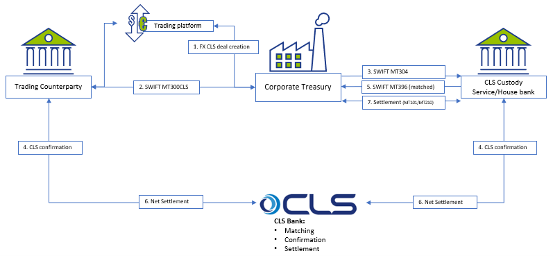
The proposed solution may be applicable for a corporate using SAP TRM (ECC to S/4HANA), having Credit risk analyzer activated and using SWIFT connection for connectivity with the banks.
Capturing CLS FX deals
There are a few options on how to register the FX deal as a CLS deal, with two described below:
Option 1: CLS Business partner – a replica of your usual business partner (BP) which would have CLS BIC code and complete settlement instructions.
Option 2: CLS FX product type/transaction type – a replica of normal FX SPOT, FX FORWARD or FX SWAP product type/transaction type.
Each option has pros and cons and may be applied as per a client technical specific.
FX deals trading and capturing may be executed via SAP Trade Platform Integration (TPI), which would improve the processing efficiency, but development may still be required depending on characteristics of the scope of FX dealing. In particular, the currency, product type, counterparty scope and volume of transactions would drive whether additional development is required, or whether standard mapping logic can be used to isolate CLS deals.
For the scenarios where a custom solution is required to convert standard FX deals into CLS FX deals during its creation, a custom program could be created that includes an additional mapping table to help SAP determine CLS eligible deals. The bespoke mapping table could help identify CLS eligibility based on the below characteristics:
- Counterparty
- Currency Pair
- Product Type (Spot, Forward, SWAP)
Correspondence framework
Once CLS deal is captured in SAP TRM, it needs to be counter-confirmed with the trading counterparty and with CLS Bank. Three new types of correspondence need to be configured:
- MT300 with CLS specifics to be used to communicate with the trading counterparty;
- MT304 to communicate with CLS Custody service;
- SWIFT MT396 to get the matching status from CLS bank.
Credit Risk Analyzer (CRA)
FX CLS deals do not bring settlement exposure, thus CLS deals need to be exempt from the settlement risk utilization. Configuration of the limit characteristics must include either business partner number (for CLS Business Partner) or transaction type (for CLS transaction type). This will help determine the limits without FX CLS deals.
No automatic limits creation should be allowed for the respective limit type; this will disable a settlement limit creation based on CLS deal capture in SAP.
CLS Business partner setting must be done with ‘parent <-> subsidiary’ relationship with the regular business partner. This is required to keep a single credit limit utilization and having FX deals being done with two business partners.
Deal execution
Accounting for CLS FX deals is normally the same as for regular FX deals, though it depends on the corporate requirements. We do not see any need for a separate FX unrealized result treatment for CLS deals.
However, settlement of CLS deals is different and standard settlement instructions of CLS deals vary from normal FX deals.
Either the bank’s virtual accounts or separate house bank accounts are opened to settle CLS FX deals.
Since CLS partner performs the net settlement on-behalf of a corporate there is no need to generate payment request for every CLS deal separately. Posting to the bank’s CLS clearing account with cash flow postings (TBB1) is sufficient at this level.
The following day the bank statement will clear the postings on the CLS settlement account on a net basis based on the total amount and posting date.
Cash Management
A liquidity manager needs to know the net result of the CLS deals in advance to replenish the CLS bank account in case the net settlement amount for CLS deal is negative. In addition, the funds would need to be transmitted between the house bank accounts either manually or automatically, with cash concentration requiring transparency on the projected cash position.
The solution may require extra settings in the cash management module with CLS bank accounts to be added to specific groupings.
Conclusion
Designing a CLS solution in SAP requires deep understanding of a client’s treasury operations, bank account structure and SAP TMS specifics. Together with a client and based on the unique business landscape, we review the pros and cons of possible solutions and help choosing the best one. Eventually we can design and implement a solution that makes treasury operations more efficient and transparent.
Our corporate clients are requesting our support with design and implementation of Continuous Linked Settlement (CLS) solutions for FX settlements in their SAP Treasury system. If you are interested, please do not hesitate to contact us.

Analyzing data from a treasury management system and ensuring it is up to date and accurate is key to making effective decisions for any corporate treasurer.
Over recent years, SAP has added an array of products in the data warehousing, reporting and analytics space to assist decision-making as well as address some of the historical weaknesses in its reporting capabilities.
These more recent SAP tools focus on delivering key business drivers in the reporting space – such as agility, flexibility, independence from IT, data processing, intelligent analysis (using artificial intelligence), and data centralization – thereby addressing many of the previous frustrations that business users experienced with getting the necessary information out of their SAP systems to make sound business decisions. Previously, reporting within SAP was often limited, inflexible and required a reliance on IT to develop custom reports and/or data models. But with more options, choosing the most appropriate reporting landscape design can seem overwhelming to the treasury executive and it’s easy to get lost in the technical jargon.
The appropriate tool for your unique business design
When it comes to treasury analytics solutions offered by SAP, there are among others embedded Fiori analytical apps, SAP Analytics Cloud, BW4/HANA and the new Data Warehouse Cloud. It may be difficult to get a clear understanding of what each tool offers and for what purposes to use each. The question then is whether to invest in all tools or which one(s) to choose to meet our reporting needs. Additionally, there may be uncertainty too around what is offered to customers using SAP S/4HANA Cloud versus those customers who run SAP S/4HANA Cloud, private edition (and on premise deployments).
The answer about how to structure your SAP reporting architecture depends on your unique business design and reporting requirements, and more specifically what questions you need answered by your data. Here we will give a brief overview of the functionality of the main tools and what to consider when making system selection decisions. Note, the below information speaks more to customers who run the on-premise version of SAP S/4HANA, although we do mention what is offered on the cloud, where relevant.
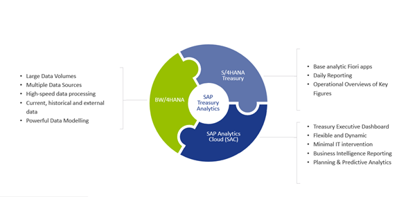
SAP S/4HANA Fiori Analytical Apps
SAP S/4HANA Finance for treasury and risk management comes standard with analytical Fiori apps for daily reporting as well as Dashboard reporting. With your daily reporting apps, you will be able to display treasury position flows, analyze the treasury position, use the Cash Flow Analyzer as well as display the treasury posting journal. These apps assist the treasury executive to see the details and results of what has taken place over a given period within the organization. There are also currently four dashboard-type Fiori apps which give an overview of different key areas, namely Foreign Exchange Overview, Interest Rate Overview, Market Data Overview, and Bank Relationship Overview.
Without paying any additional license fees, the above apps give the treasury executive a great starting point with which to review current positions but may not be sufficient to provide the information you want to see and how you want to see it.
SAP Analytics Cloud
SAP Analytics Cloud is SAP’s solution for data visualization, offering business intelligence, planning and predictive analytics in a single solution for all modules, providing a broader, deeper and more flexible analysis of the organization’s operations than the embedded analytical Fiori apps can.
Although the SAP Analytics Cloud OEM version is delivered embedded into Treasury Management for SAP S/4HANA Cloud, customers with the SAP S/4HANA Cloud, private edition, or an on-premise version of Treasury Management will need an additional license to get access to SAP Analytics Cloud functionality. However, it is worth noting that this license is for the full-use SAP Analytics Cloud Enterprise edition, which comes with more features and functionalities than the embedded version.
In terms of Treasury Management, the Treasury Executive Dashboard is the main offering within SAP Analytics Cloud. This dashboard is based on a preconfigured data model that offers real-time insights into the treasury operations across eight tab strips. Areas that can be reported on are Liquidity, Cash management, Bank relationship, Indebtedness, Counterparty risk, Market risk, Bank guarantee and Market overview. The dashboard provides visual overviews of the underlying data and allows for drill-down to see the detail. Customizing the layout is also possible.
With the full-use Enterprise version of SAP Analytics Cloud, there is the possibility of creating more dashboards (called Stories) according to business reporting needs. Business Content is also delivered out the box with the full version which means the creation of new dashboards is accelerated as the groundwork has already been done by SAP or one of their business partners.
Another feature of SAP Analytics Cloud worth mentioning is its predictive capabilities. Historical data is analyzed to identify trends and patterns, and these are then used to predict a potential future outcome, further adding to the tools at the executive’s disposal.
SAP Analytics Cloud is designed to be set up and used by the business user with minimal IT intervention. Dashboards are responsive and user-friendly, with a large degree of flexibility in terms of layout and design.
SAP BW/4HANA
SAP BW/4HANA is SAP’s next generation data warehousing solution designed to run exclusively on the SAP HANA database. The key areas of focus for SAP BW∕4HANA are data modeling, data procurement, analysis and planning. An SAP customer needs to license this product and it runs on a separate instance.
SAP BW/4HANA is not an upgrade of SAP BW but a widely rewritten solution designed to reduce complexity and effort around data warehousing as well as increasing speed and agility, offering advanced UIs.
Data from multiple sources across the enterprise can be imported and stored centrally in the SAP BW∕4HANA Enterprise Data Warehouse. This data can be transformed and cleaned up, ready for analysis. SAP BW/4HANA provides a single source of truth, handling large data volumes at speed for complex organizations. SAP BW/4HANA has been designed to create reports on current, historical, and external data from multiple SAP and non-SAP sources. The data modeling capabilities are also much more powerful than SAP Analytics Cloud offers as a standalone solution.
A note here that SAP has recently released the Data Warehouse Cloud. This is intended as a data warehousing solution for SAP S/4HANA Cloud customers and is not seen as a direct replacement for BW/4HANA. However, the approaches for supporting Self-Service BI, the “SAP BW Bridge capabilities”, or the inclusion of CDS views from SAP S/4HANA make it a good candidate for a hybrid approach at least.
Selecting the right solution
SAP believes that there are four main drivers of the value of data – Span (data from anywhere), Volume (data of any size), Quality (data of any kind) and Usage (data for anyone). They have focused on ensuring that value is maximized for organizations by offering solutions for each driver. The SAP HANA database ensures that a vast volume of data can be handled at high speed, SAP BW/4HANA has been designed so that high volumes of data of any kind can be consolidated for analysis and SAP Analytics Cloud delivers a single solution for visual, easy-to-use analytics across the business.
Customers that have SAP S/4HANA Treasury in their on-premise deployment with minimal data sources could supplement their SAP S/4HANA Treasury system with SAP Analytics Cloud alone. This is ideal when the main reporting needs are operational and real-time and would allow treasury executives to easily access the information they need to optimize their portfolios for liquidity and risk, giving them the additional flexibility and ability to design required reports.
Where the data volumes are large and from a diverse range of sources, a combination of SAP BW4/HANA and SAP Analytics Cloud could be better. The latter has been optimized to work with SAP BW/4HANA as a source and this allows customers to get the powerful, interactive visualizations of SAP Analytics Cloud using the immense data volume capabilities of SAP BW/4HANA. Together, these two products, alongside your SAP S/4HANA Treasury system, give up-to-date, broad, easy-to-read information at a glance to ensure the treasury executive can be proactive and responsive, making the best possible decisions around liquidity, funding and risk management across the entire enterprise. SAP BW4/HANA can of course be implemented without SAP Analytics Cloud, as other BI tools can be used, but the advantages of SAP Analytics Cloud are the highly visual design, flexibility and most importantly not needing to rely on IT to design reports.
To conclude
Knowing what your options are and which would suit your current and future system landscapes is where Zanders can come in, providing sound guidance and ensuring you are able to make the most of any investment to analyze data and make decisions. We can assist treasury executives by ensuring the customer has the right mix of reporting solutions, weighing up total cost of ownership against the data reporting requirements of the organization.

Continuous Linked Settlement (CLS) is an established global system to mitigate settlement risks for FX trades, improving corporate cash and liquidity management among other benefits. The CLS system was established back in 2002 and since then, the FX market has grown significantly. Therefore, there is a high demand from corporates to leverage CLS to improve corporate treasury efficiency.
In this article we shed some light on the possible technical solutions in SAP Treasury to implement CLS in the corporate treasury operations. This includes CLS deal capture, limit utilization implications in Credit risk analyzer, and changes in the correspondence framework of SAP TRM.
Technical solution in SAP Treasury
There is no SAP standard solution for CLS as such. However, SAP standard functionality can be used to cover major parts of the CLS solution. The solution may vary depending on the existing functionality for hedge management/accounting and limit management as well as the technical landscape accounting for SAP version and SWIFT connectivity.
Below is a simplified workflow of CLS deal processing:

The proposed solution may be applicable for a corporate using SAP TRM (ECC to S/4HANA), having Credit risk analyzer activated and using SWIFT connection for connectivity with the banks.
Capturing CLS FX deals
There are a few options on how to register the FX deal as a CLS deal, with two described below:
Option 1: CLS Business partner – a replica of your usual business partner (BP) which would have CLS BIC code and complete settlement instructions.
Option 2: CLS FX product type/transaction type – a replica of normal FX SPOT, FX FORWARD or FX SWAP product type/transaction type.
Each option has pros and cons and may be applied as per a client technical specific.
FX deals trading and capturing may be executed via SAP Trade Platform Integration (TPI), which would improve the processing efficiency, but development may still be required depending on characteristics of the scope of FX dealing. In particular, the currency, product type, counterparty scope and volume of transactions would drive whether additional development is required, or whether standard mapping logic can be used to isolate CLS deals.
For the scenarios where a custom solution is required to convert standard FX deals into CLS FX deals during its creation, a custom program could be created that includes an additional mapping table to help SAP determine CLS eligible deals. The bespoke mapping table could help identify CLS eligibility based on the below characteristics:
- Counterparty
- Currency Pair
- Product Type (Spot, Forward, SWAP)
Correspondence framework
Once CLS deal is captured in SAP TRM, it needs to be counter-confirmed with the trading counterparty and with CLS Bank. Three new types of correspondence need to be configured:
- MT300 with CLS specifics to be used to communicate with the trading counterparty;
- MT304 to communicate with CLS Custody service;
- SWIFT MT396 to get the matching status from CLS bank.
Credit Risk Analyzer (CRA)
FX CLS deals do not bring settlement exposure, thus CLS deals need to be exempt from the settlement risk utilization. Configuration of the limit characteristics must include either business partner number (for CLS Business Partner) or transaction type (for CLS transaction type). This will help determine the limits without FX CLS deals.
No automatic limits creation should be allowed for the respective limit type; this will disable a settlement limit creation based on CLS deal capture in SAP.
CLS Business partner setting must be done with ‘parent <-> subsidiary’ relationship with the regular business partner. This is required to keep a single credit limit utilization and having FX deals being done with two business partners.
Deal execution
Accounting for CLS FX deals is normally the same as for regular FX deals, though it depends on the corporate requirements. We do not see any need for a separate FX unrealized result treatment for CLS deals.
However, settlement of CLS deals is different and standard settlement instructions of CLS deals vary from normal FX deals.
Either the bank’s virtual accounts or separate house bank accounts are opened to settle CLS FX deals.
Since CLS partner performs the net settlement on-behalf of a corporate there is no need to generate payment request for every CLS deal separately. Posting to the bank’s CLS clearing account with cash flow postings (TBB1) is sufficient at this level.
The following day the bank statement will clear the postings on the CLS settlement account on a net basis based on the total amount and posting date.
Cash Management
A liquidity manager needs to know the net result of the CLS deals in advance to replenish the CLS bank account in case the net settlement amount for CLS deal is negative. In addition, the funds would need to be transmitted between the house bank accounts either manually or automatically, with cash concentration requiring transparency on the projected cash position.
The solution may require extra settings in the cash management module with CLS bank accounts to be added to specific groupings.
Conclusion
Designing a CLS solution in SAP requires deep understanding of a client’s treasury operations, bank account structure and SAP TMS specifics. Together with a client and based on the unique business landscape, we review the pros and cons of possible solutions and help choosing the best one. Eventually we can design and implement a solution that makes treasury operations more efficient and transparent.
Our corporate clients are requesting our support with design and implementation of Continuous Linked Settlement (CLS) solutions for FX settlements in their SAP Treasury system. If you are interested, please do not hesitate to contact us.

Everyone understands the importance of data in an organization. After all, data is the new oil in terms of its value to a corporate treasury and indeed the wider organization. However, not everyone is aware of how best to utilize data. This article will tell you.
Developing a data strategy depends on using the various types of payment, market, cashflow, bank and risk data available to a treasury, and then considering the time implications of past historical data, present and future models, to better inform decision-making. We provide a roadmap and ‘how to’ guide to becoming a data-driven organization.
Why does this aim matter? Well, in this age of digitization, almost every aspect of the business has a digital footprint. Some significantly more than the others. This presents a unique opportunity where potentially all information can be reliably processed to take tactical and strategic decisions from a position of knowledge. Good data can facilitate hedging, forecasting and other key corporate activities. Having said all that, care must also be taken to not drown in the data lake1 and become over-burdened with useless information. Take the example of Amazon in 2006 when it reported that cross-selling attributed for 35% of their revenue2. This strategy looked at data from shopping carts and recommended other items that may be of interest to the consumer. The uplift in sales was achieved only because Amazon made the best use of their data.
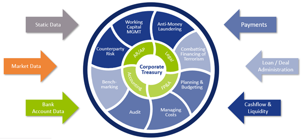
Treasury is no exception. It too can become data-driven thanks to its access to multiple functions and information flows. There are numerous ways to access and assess multiple sets of data (see Figure 1), thereby finding solutions to some of the perennial problems facing any organization that wants to mitigate or harness risk, study behavior, or optimize its finances and cashflow to better shape its future.
Time is money
The practical business use cases that can be realized by harnessing data in the Treasury often revolve around mastering the time function. Cash optimization, pooling for interest and so on often depend on a good understanding of time – even risk hedging strategies can depend on the seasons, for instance, if we’re talking about energy usage.
When we look at the same set of data from a time perspective, it can be used for three different purposes:
I. Understand the ‘The Past’ – to determine what transpired,
II. Ascertain ‘The Present’ situation,
III. Predict ‘The Future’ based on probable scenarios and business projections.
I – The Past
“Study the past if you would define the future”
Confucius

The data in an organization is the undeniable proof of what transpired in the past. This fact makes it ideal to perform analysis through Key Performance Indicators (KPIs), perform statistical analysis on bank wallet distribution & fee costs, and it can also help to find the root cause of any irregularities in the payments arena. Harnessing historical data can also positively impact hedging strategies.
II – The Present
“The future depends on what we do in the present”
M Gandhi
Data when analyzed in real-time can keep stakeholders updated and more importantly provide a substantial basis for taking better informed tactical decisions. Things like exposure, limits & exceptions management, intra-day cash visibility or near real-time insight/access to global cash positions all benefit, as does payment statuses which are particularly important for day-to-day treasury operations.
III – The Future
“The best way to predict the future is to create it.”
Abraham Lincoln
There are various areas where an organization would like to know how it would perform under changing conditions. Simulating outcomes and running future probable scenarios can help firms prepare better for the near and long-term future.
These forecast analyses broadly fall under two categories:
Historical data: assumes that history repeats itself. Predictive analytics on forecast models therefore deliver results.
Probabilistic modeling: this creates scenarios for the future based on the best available knowledge in the present.
Some of the more standard uses of forecasting capabilities include:
- risk scenarios analysis,
- sensitivity analysis,
- stress testing,
- analysis of tax implications on cash management structures across countries,
- & collateral management based on predictive cash forecasting, adjusted for different currencies.
Working capital forecasting is also relevant, but has typically been a complex process. The predication accuracy can be improved by analyzing historical trends and business projections of variables like receivables, liabilities, payments, collections, sales, and so on. These can feed the forecasting algorithms. In conjunction with analysis of cash requirements in each business through studying the trends in key variables like balances, intercompany payments and receipts, variance between forecasts and actuals, this approach can lead to more accurate working capital management.
How to become a data-driven organization
“Data is a precious thing and will last longer than the systems themselves.”
Tim Berners-Lee
There can be many uses of data. Some may not be linked directly to the workings of the treasury or may not even have immediate tangible benefits, although they might in the future for comparative purposes. That is why data is like a gold mine that is waiting to be explored. However, accessing it and making it usable is a challenging proposition. It needs a roadmap.
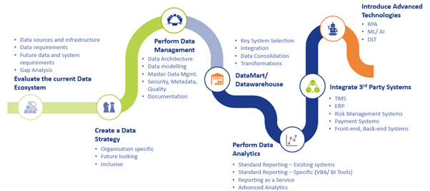
The most important thing that can be done in the beginning is to perform a gap analysis of the data ecosystem in an organization and to develop a data strategy, which would embed importance of data into the organization’s culture. This would then act as a catalyst for treasury and organizational transformation to reach the target state of being data-driven.
The below roadmap offers a path to corporates that want to consistently make the best use of one of their most critical and under-appreciated resources – namely, data.
We have seen examples like Amazon and countless others where organizations have become data- driven and are reaping the benefits. The same can be said about some of the best treasury departments we at Zanders have interacted with. They are already creating substantial value by analyzing and making the optimum use of their digital footprint. The best part is that they are still on their journey to find better uses of data and have never stopped innovating.
The only thing that one should be asking now is: “Do we have opportunities to look at our digital footprint and create value (like Amazon did), and how soon can we act on it?”
References:

Over the past years, more and more corporates have implemented a sustainability framework, incorporating specific KPIs that can be used as a basis to arrange sustainability-linked funding instruments.
Next to sustainable funding instruments, including both green and social, we also see that these KPI’s can be used for other financial instruments, such as ESG (Environmental, Social, Governance) derivatives. These derivatives are a useful tool to further drive the corporate sustainability strategy or support meeting environmental targets.
Since the first sustainability-linked derivative was executed in 2019, market participants have entered into a variety of ESG-related derivatives and products. In this article we provide you with an overview of the different ESG derivatives. We will touch upon the regulatory and valuation implications of this relatively new derivative class in a subsequent article, which will be published later this year.
Types of ESG-related derivatives products
Driven by regulatory pressure and public scrutiny, corporates have been increasingly looking for ways to manage their sustainability footprint. As a result of a blooming ESG funding market, the role of derivatives to help meet sustainability goals has grown. ESG-related derivatives cover a broad spectrum of derivative products such as forwards, futures and swaps. Five types (see figure 1) of derivatives related to ESG can be identified; of which three are currently deemed most relevant from an ESG perspective.
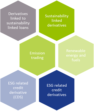
The first category consists of traditional derivatives such as interest rate swaps or cross currency swaps that are linked to a sustainable funding instrument. The derivative as such does not contain a sustainability element.
Sustainability-linked derivatives
Sustainability-linked derivatives are agreements between two counterparties (let’s assume a bank and a corporate) which contain a commitment of the corporate counterparty to achieve specific sustainability performance targets. When the sustainability performance targets are met by the corporate during the lifetime of the derivative, a discount is applied by the bank to the hedging instrument. When the targets are not met, a premium is added. Usually, banks invest the premium they receive in sustainable projects or investments. Sustainability-linked derivative transactions are highly customizable and use tailor-made KPIs to determine sustainability goals. Sustainability-linked derivatives provide market participants with a financial incentive to improve their ESG performance. An example is Enel’s sustainability-linked cross currency swap, which was executed in July 2021 to hedge their USD/EUR exchange rate and interest rate exposures.
Emission trading derivatives
Other ESG-related derivatives support meeting sustainable business models and consist of trading carbon offsets, emission trading derivatives, and renewable energy and renewable fuels derivatives, amongst others. Contrary to sustainability-linked derivatives, the use of proceeds of ESG-related derivatives are allocated to specific ESG-related purposes. For example, emissions trading is a market-based approach to reduce pollution by setting a (geographical) limit on the amount of greenhouse gases that can be emitted. It consists of a limit or cap on pollution and tradable instruments that authorize holders to emit a specific quantity of the respective greenhouse gas. Market participants can trade derivatives based on emission allowances on exchanges or OTC markets as spots, forwards, futures and option contracts. The market consists of mandatory compliance schemes and voluntary emission reduction programs.
Renewable energy and fuel derivatives
Another type of ESG-related derivatives are renewable energy and renewable fuel hedging transactions, which are a valuable tool for market participants to hedge risks associated with fluctuations in renewable energy production. These ESG-related credit derivatives encourage more capital to be contributed to renewable energy projects. Examples are Power Purchase Agreements (PPAs), Renewable Energy Certificate (REC) futures, wind index futures and low carbon fuel standard futures.
ESG related credit derivatives
ESG-related CDS products can be used to manage the credit risk of a counterparty when financial results may be impacted by climate change or, more indirectly, if results are affected due to substitution of a specific product/service. An example of this could be in the airline industry where short-haul flights may be replaced by train travel. Popularity of ESG-related CDS products will probably increase with the rising perception that companies with high ESG ratings exhibit low credit risk.
Catastrophe and weather derivatives
Catastrophe and weather derivatives are insurance-like products as well. Both markets have existed for several decades and are used to hedge exposures to weather or natural disasters. Catastrophe derivatives are financial instruments that allow for transferral of natural disaster risk between market participants. These derivatives are traded on OTC markets and enable protection from enormous potential losses following from natural disasters such as earthquakes to be obtained. The World Bank has designed catastrophe swaps that support the transfer of risks related to natural disasters by emerging countries to capital markets. An example if this is the swap issued for the Philippines in 2017. Weather derivatives are financial instruments that derive their value from weather-related factors such as temperature and wind. There derivatives are used to mitigate risks associated with adverse or unexpected weather conditions and are most commonly used in the food and agriculture industry.
What’s old, what’s new and what’s next?
ESG-related credit derivatives would be best applied by organizations with credit exposures to certain industries and financial institutions. Despite the link to an environmental element, we do not consider catastrophe bonds and weather derivatives as a sustainability-linked derivative. Neither is it an innovative, new product that is applicable to corporates in various sectors.
Truly innovative products are sustainability-linked derivatives, voluntary emissions trading and renewable energy and fuel derivatives. These products strengthen a corporate’s commitment to meet sustainability targets or support investments in sustainable initiatives. A lack of sustainability regulation for derivatives raises the question to what extent these innovative products are sustainable on their own? An explicit incentive for financial institutions to execute ESG-related derivatives, such as a capital relief, is currently absent. This implies that any price advantage will be driven by supply and demand.
Corporate Treasury should ensure they consider the implications of using ESG-related derivatives that affect the cashflows of derivatives transactions. Examples of possible regulatory obligations consist of valuation requirements, dispute resolution and reporting requirements. Since ESG-related derivatives and products are here to stay, Zanders recommends that corporate treasurers closely monitor the added value of specific instruments, as well as the regulatory, tax and accounting implications. Part II of this series, later in the year, will focus on the regulatory and valuation implications of this relatively new derivative class.
For more information on ESG issues, please contact Sander van Tol.


On 24 January 2022, the European Banking Authority (EBA) published its final draft Implementing Technical Standards (ITS) on Pillar 3 (P3) disclosures on Environmental, Social and Governance (ESG) risks.
This publication fits nicely into the ‘horizon priority’ of the EBA1 to provide tools to banks to measure and manage ESG-related risks. In this article we present a brief overview of the way the ITS have been developed, what qualitative and quantitative disclosures are required, what timelines and transitional measures apply – and where the largest challenges arise. By requiring banks to disclose information on their exposure to ESG-related risks and the actions they take to mitigate those risks – for example by supporting their clients and counterparties in the adaptation process – the EBA wants to contribute to a transition to a more sustainable economy. The Pillar 3 disclosure requirements apply to large institutions with securities traded on a regulated market of an EU member state.
In an earlier report2, the EBA defined ESG-related risks as “the risks of any negative financial impact on the institution stemming from the current or prospective impacts of ESG factors on its counterparties or invested assets”. Hence, the focus is not on the direct impact of ESG factors on the institution, but on the indirect impact through the exposure of counterparties and invested assets to ESG-related risks. The EBA report also provides examples for typical ESG-related factors.
While the ITS have been streamlined and simplified compared to the consultation paper published in March 2021, there are plenty of challenges remaining for banks to implement these standards.
Development of the ITS
The EBA has been mandated to develop the ITS on P3 disclosures on ESG risks in Article 434a of the Capital Requirements Regulation (CRR). The EBA has opted for a sequential approach, with an initial focus on climate change-related risks. This is further narrowed down by only considering the banking book. The short maturity and fast revolving positions in the trading book are out of scope for now. The scope of the ITS will be extended to included other environmental risks (like loss of biodiversity), and social and governance risks, in later stages.
In the development of the ITS, the EBA has strived for alignment with several other regulations and initiatives on climate-related disclosures that apply to banks. The most notable ones are listed below (and in Figure 1):

Figure 1 – Overview of related regulations and initiatives considered in the development of the ITS
- Capital Requirements Directive and Regulation (CRD and CRR): article 98(8) of the CRD3 mandated the EBA to publish the EBA report on Management and Supervision of ESG risks, which includes the split of climate change-related risks in physical and transition risks. Article 434a of the CRR4 mandated the EBA to develop the draft ITS to specify the ESG disclosure requirements described in article 449a.
- EBA report on Management and Supervision of ESG risks2: the report provides common definitions of ESG risks and contains proposals on how to include ESG risks in the risk frameworks of banks, covering its identification, assessment, and management. It also discusses the way to include ESG risks in the supervisory review process.
- Task Force on Climate-related Financial Disclosures (TCFD)5: the Financial Stability Board’s TFCD has published recommendations on climate-related disclosures. The metrics and Key Performance Indicators (KPIs) included in the ITS have been aligned with the TCFD recommendations.
- Taxonomy Regulation6: the European Union’s common classification system of environmentally sustainable economic activities is underpinning the main KPIs introduced in the ITS.
- Climate Benchmark Regulation (CBR)7: In the CBR, two types of climate benchmarks were introduced (‘EU Climate Transition’ and ‘EU Paris-aligned’ benchmarks) and ESG disclosures for all other benchmarks (excluding interest rate and currency benchmarks) were required.
- Non-Financial Reporting Directive (NFRD)8: the NFRD introduces ESG disclosure obligations for large companies, which include climate-related information.
- Corporate Sustainability Reporting Directive (CSRD)9: a proposal by the European Commission to extend the scope of the NFRD to also include all companies listed on regulated markets (except listed micro-enterprises). One of the ITS’s KPIs, the Green Asset Ratio (GAR) is directly linked to the scope of the NFRD/CSRD.
- Sustainable Finance Disclosure Regulation (SFDR)10: the SFDR lays down sustainability disclosure obligations for manufacturers of financial products and financial advisers towards end-investors. It applies to banks that provide portfolio management investment advice services.
Compared to the consultation paper for the ITS, several changes have been made to the required templates. Some templates have been combined (e.g., templates #1 and #2 from the consultation paper have been combined into template #1 of the final draft ITS) and several templates have been reorganized and trimmed down (e.g., the requirement to report exposures to top EU or top national polluters has been removed).
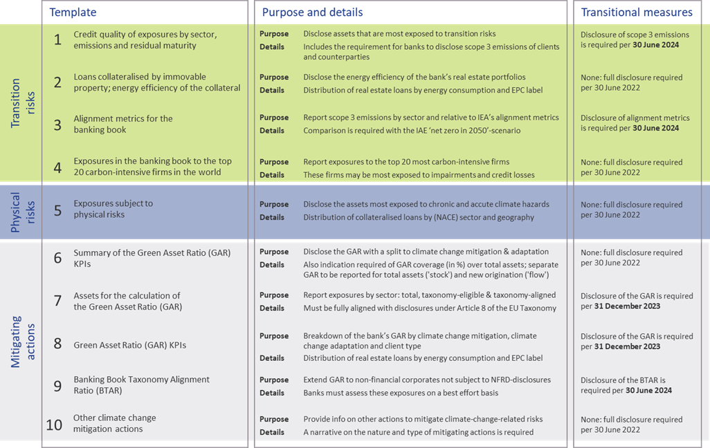
Quantitative disclosures
The ITS on P3 disclosure on ESG risks introduce ten templates on quantitative disclosures. These can be grouped in four templates on transition risks, one on physical risks, and five on mitigating actions:
- Transition risks
Two of the required templates are relatively straightforward. Banks need to report the energy efficiency of real estate collateral in the loan portfolio (#2) and report their aggregate exposure to the top 20 of the most carbon-intensive firms in the world (#4).
The main challenge for banks though will be in completing the other two templates:- Template #1 requires banks to disclose the gross carrying amount of loans and advances provided to non-financial corporates, classified by NACE sector codes and residual maturities. It is also required to report on the counterparties’ scope 1, 2, and 3 greenhouse gas (GHG) emissions. Reflecting the challenge in reporting on scope 3 emissions, a transitional measure is in place. Full reporting needs to be in place by June 2024. Until then, banks need to report their available estimates (if any) and explain the methodologies and data sources they intend to use.
- In the last template (#3), banks also need to report scope 3 emissions, but relate these to the alignment metrics defined by the International Energy Agency (IEA) for the ‘net zero by 2050’ scenario. For this scenario, a target for a CO2 intensity metric is defined for 2030. By calculating the distance to this target, it becomes clear how banks are progressing (over time) towards supporting a sustainable economy. A similar transitional measure applies as for template #1.
- Physical risks
In template #5, banks are required to disclose how their banking book positions are exposed to physical risks, i.e., “chronic and acute climate-related hazards”. The exposures need to be reported by residual maturity and by NACE sector codes and should reflect exposure to risks like heat waves, droughts, floods, hurricanes, and wildfires. Specialized databases need to be consulted to compile a detailed understanding of these exposures. To support their submissions, banks further need to compile a narrative that explains the methodologies they used. - Mitigating actions
The final set of templates covers quantitative information on the actions a bank takes to mitigate or adapt to climate change risks.- Templates #6-8 all relate to the GAR, which indicates what part of the bank’s banking book is aligned with the EU’s Taxonomy:
- In template #7, banks need to report the outstanding banking book exposures to different types of clients/issuers, as well as the amount of these exposures that are taxonomy-eligible (that is, to sectors included in the EU Taxonomy) and taxonomy-aligned (that is, taxonomy-eligible exposures financing activities that contribute to climate change mitigation or adaptation). Based on this information, the bank’s GAR can be determined.
- In template #8, a GAR needs to be reported for the exposures to each type of client/issuer distinguished in template #7, with a distinction between a GAR for the full outstanding stock of exposures per client/issuer type, and a GAR for newly originated (‘flow’) exposures.
- Template #6 contains a summary of the GARs from templates #7 and #8.
In these templates, the numerator of the GAR only includes exposures to non-financial corporations that are required to publish non-financial information under the NFRD. Any exposures to other corporate counterparties therefore are considered 0% Taxonomy-aligned.
- The main challenge in this group of templates is in template #9. To incentivize banks to support all of their counterparties to transition to a more sustainable business model, and to collect ESG data on these counterparties, the EBA introduces the Banking Book Taxonomy Alignment Ratio (BTAR). In this metric, the numerator does include the exposures to counterparties that are not subject to NFRD disclosure obligations. The BTAR ratios obtained from the information in template #9 therefore complement the GAR ratios obtained in templates #7 and #8.
- In the final template (#10), banks have the opportunity to include any other climate change mitigating actions that are not covered by the EU Taxonomy. They can for example report on their use of green or sustainable bonds and loans.
- Templates #6-8 all relate to the GAR, which indicates what part of the bank’s banking book is aligned with the EU’s Taxonomy:
An overview of the templates for quantitative disclosures in presented in Figure 2.
Qualitative disclosures
In the ITS on P3 disclosures on ESG risks, three tables are included for qualitative disclosures. The EBA has aligned these tables with their Report on Management and Supervision of ESG risks11. The three tables are set up for qualitative information on environmental, social, and governance risks, respectively. For each of these topics, banks need to address three aspects: on business strategy and processes, governance, and risk management. An overview of the required disclosures is presented in Figure 3.
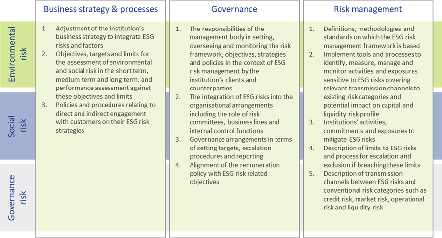
Figure 3 – Overview of qualitative ESG disclosures (based on templates & section 2.3.2 of the EBA ITS on P3 disclosures on ESG risks)
Timelines and transitional measures
The ITS on P3 disclosure on ESG risks become effective per 30 June 2022 for large institutions that have securities traded on a regulated market of an EU member state. A semi-annual disclosure is required, but the first disclosure is annual. Consequently, based on 31 December 2022 data, the first reporting will take place in the first quarter of 2023.
The EBA has introduced a number of transitional measures. These can be summarized as follows:
- The reporting of information on the GAR is only required as of 31 December 2023.
- The reporting of information on the BTAR, the bank’s financed scope 3 emissions, and the alignment metrics is only required as of June 2024.
The EBA has further indicated in the ITS that they will conduct a review of the ITS’s requirements during 2024. They may then also extend the ITS with other environmental risks (other than the climate change-related risks in the current version). The EU Taxonomy is expected to cover a broader range of environmental risks by the end of 2022. Sometime after 2024, it is expected that the EBA will further extend the ITS by including disclosure requirements on social and governance risks.
An overview of the main timelines and transitional measures is presented in Figure 4.
Figure 4 – Overview of the main timelines and transitional measures for the ESG disclosures
Conclusion
Society, and consequently banks too, are increasingly facing risks stemming from changes in our climate. In recent years, supervisory authorities have stepped up by introducing more and more guidance and regulation to create transparency about climate change risk, and more broadly ESG risks. The publication of the ITS on P3 disclosures on ESG risks by the EBA marks an important milestone. It offers banks the opportunity to disseminate a constructive and positive role in the transition to a sustainable economy.
Nonetheless, implementing the disclosure requirements will be a challenge. Developing detailed assessments of the physical risks to which their asset portfolio is exposed and to estimate the scope 3 emissions of their clients and counterparties (‘financed emissions’) will not be straightforward. For their largest counterparties, banks will be able to profit from the NFRD disclosure obligations, but especially in Europe a bank’s portfolio typically has many exposures to small- and medium-sized enterprises. Meeting the disclosure requirements introduced by the EBA will require timely and intensive discussions with a substantial part of the bank’s counterparties.
Banks also need to provide detailed information on how ESG risks are reflected in the bank’s strategy and governance and incorporated in the risk management framework. With our extensive knowledge on market risk, credit risk, liquidity risk, and business risk, Zanders is well equipped to support banks with integrating the identification, measurement, and management of climate change-related risks into existing risk frameworks. For more information, please contact Pieter Klaassen or Sjoerd Blijlevens via +31 88 991 02 00.
References
- See the EBA 2022 Work Programme.
- The EBA’s Report on Management and Supervision of ESG risks for credit institutions and investment firms, published in June 2021.
- See the EBA’s interactive Single Rulebook.
- See Regulation (EU) 2019/876.
- See the TCFD’s Final Report on Recommendations of the Task Force on Climate-related Financial Disclosures published in June 2017.
- See the EBA’s response to EC Call for Advice on Article 8 Taxonomy Regulation.
- See Regulation (EU) 2019/2089.
- See Directive 2014/95/EU.
- See the European Commission’s Proposal for a Corporate Sustainability Reporting Directive.
- See Regulation (EU) 2019/2088.
- The EBA report can be found here.

On 24 January 2022, the European Banking Authority (EBA) published its final draft Implementing Technical Standards (ITS) on Pillar 3 (P3) disclosures on Environmental, Social and Governance (ESG) risks.
This publication fits nicely into the ‘horizon priority’ of the EBA to provide tools to banks to measure and manage ESG-related risks. In this article we present a brief overview of the way the ITS have been developed, what qualitative and quantitative disclosures are required, what timelines and transitional measures apply – and where the largest challenges arise.
By requiring banks to disclose information on their exposure to ESG-related risks and the actions they take to mitigate those risks – for example by supporting their clients and counterparties in the adaptation process – the EBA wants to contribute to a transition to a more sustainable economy. The Pillar 3 disclosure requirements apply to large institutions with securities traded on a regulated market of an EU member state.
In an earlier report2, the EBA defined ESG-related risks as “the risks of any negative financial impact on the institution stemming from the current or prospective impacts of ESG factors on its counterparties or invested assets”. Hence, the focus is not on the direct impact of ESG factors on the institution, but on the indirect impact through the exposure of counterparties and invested assets to ESG-related risks. The EBA report also provides examples for typical ESG-related factors.
While the ITS have been streamlined and simplified compared to the consultation paper published in March 2021, there are plenty of challenges remaining for banks to implement these standards.
Development of the ITS
The EBA has been mandated to develop the ITS on P3 disclosures on ESG risks in Article 434a of the Capital Requirements Regulation (CRR). The EBA has opted for a sequential approach, with an initial focus on climate change-related risks. This is further narrowed down by only considering the banking book. The short maturity and fast revolving positions in the trading book are out of scope for now. The scope of the ITS will be extended to included other environmental risks (like loss of biodiversity), and social and governance risks, in later stages.
In the development of the ITS, the EBA has strived for alignment with several other regulations and initiatives on climate-related disclosures that apply to banks. The most notable ones are listed below (and in Figure 1):

Figure 1 – Overview of related regulations and initiatives considered in the development of the ITS
- Capital Requirements Directive and Regulation (CRD and CRR): article 98(8) of the CRD3 mandated the EBA to publish the EBA report on Management and Supervision of ESG risks, which includes the split of climate change-related risks in physical and transition risks. Article 434a of the CRR4 mandated the EBA to develop the draft ITS to specify the ESG disclosure requirements described in article 449a.
- EBA report on Management and Supervision of ESG risks2: the report provides common definitions of ESG risks and contains proposals on how to include ESG risks in the risk frameworks of banks, covering its identification, assessment, and management. It also discusses the way to include ESG risks in the supervisory review process.
- Task Force on Climate-related Financial Disclosures (TCFD)5: the Financial Stability Board’s TFCD has published recommendations on climate-related disclosures. The metrics and Key Performance Indicators (KPIs) included in the ITS have been aligned with the TCFD recommendations.
- Taxonomy Regulation6: the European Union’s common classification system of environmentally sustainable economic activities is underpinning the main KPIs introduced in the ITS.
- Climate Benchmark Regulation (CBR)7: In the CBR, two types of climate benchmarks were introduced (‘EU Climate Transition’ and ‘EU Paris-aligned’ benchmarks) and ESG disclosures for all other benchmarks (excluding interest rate and currency benchmarks) were required.
- Non-Financial Reporting Directive (NFRD)8: the NFRD introduces ESG disclosure obligations for large companies, which include climate-related information.
- Corporate Sustainability Reporting Directive (CSRD)9: a proposal by the European Commission to extend the scope of the NFRD to also include all companies listed on regulated markets (except listed micro-enterprises). One of the ITS’s KPIs, the Green Asset Ratio (GAR) is directly linked to the scope of the NFRD/CSRD.
- Sustainable Finance Disclosure Regulation (SFDR)10: the SFDR lays down sustainability disclosure obligations for manufacturers of financial products and financial advisers towards end-investors. It applies to banks that provide portfolio management investment advice services.
Compared to the consultation paper for the ITS, several changes have been made to the required templates. Some templates have been combined (e.g., templates #1 and #2 from the consultation paper have been combined into template #1 of the final draft ITS) and several templates have been reorganized and trimmed down (e.g., the requirement to report exposures to top EU or top national polluters has been removed).
Quantitative disclosures
The ITS on P3 disclosure on ESG risks introduce ten templates on quantitative disclosures. These can be grouped in four templates on transition risks, one on physical risks, and five on mitigating actions:
- Transition risks
Two of the required templates are relatively straightforward. Banks need to report the energy efficiency of real estate collateral in the loan portfolio (#2) and report their aggregate exposure to the top 20 of the most carbon-intensive firms in the world (#4).
The main challenge for banks though will be in completing the other two templates:- Template #1 requires banks to disclose the gross carrying amount of loans and advances provided to non-financial corporates, classified by NACE sector codes and residual maturities. It is also required to report on the counterparties’ scope 1, 2, and 3 greenhouse gas (GHG) emissions. Reflecting the challenge in reporting on scope 3 emissions, a transitional measure is in place. Full reporting needs to be in place by June 2024. Until then, banks need to report their available estimates (if any) and explain the methodologies and data sources they intend to use.
- In the last template (#3), banks also need to report scope 3 emissions, but relate these to the alignment metrics defined by the International Energy Agency (IEA) for the ‘net zero by 2050’ scenario. For this scenario, a target for a CO2 intensity metric is defined for 2030. By calculating the distance to this target, it becomes clear how banks are progressing (over time) towards supporting a sustainable economy. A similar transitional measure applies as for template #1.
- Physical risks
In template #5, banks are required to disclose how their banking book positions are exposed to physical risks, i.e., “chronic and acute climate-related hazards”. The exposures need to be reported by residual maturity and by NACE sector codes and should reflect exposure to risks like heat waves, droughts, floods, hurricanes, and wildfires. Specialized databases need to be consulted to compile a detailed understanding of these exposures. To support their submissions, banks further need to compile a narrative that explains the methodologies they used. - Mitigating actions
The final set of templates covers quantitative information on the actions a bank takes to mitigate or adapt to climate change risks.- Templates #6-8 all relate to the GAR, which indicates what part of the bank’s banking book is aligned with the EU’s Taxonomy:
- In template #7, banks need to report the outstanding banking book exposures to different types of clients/issuers, as well as the amount of these exposures that are taxonomy-eligible (that is, to sectors included in the EU Taxonomy) and taxonomy-aligned (that is, taxonomy-eligible exposures financing activities that contribute to climate change mitigation or adaptation). Based on this information, the bank’s GAR can be determined.
- In template #8, a GAR needs to be reported for the exposures to each type of client/issuer distinguished in template #7, with a distinction between a GAR for the full outstanding stock of exposures per client/issuer type, and a GAR for newly originated (‘flow’) exposures.
- Template #6 contains a summary of the GARs from templates #7 and #8.
In these templates, the numerator of the GAR only includes exposures to non-financial corporations that are required to publish non-financial information under the NFRD. Any exposures to other corporate counterparties therefore are considered 0% Taxonomy-aligned.
- The main challenge in this group of templates is in template #9. To incentivize banks to support all of their counterparties to transition to a more sustainable business model, and to collect ESG data on these counterparties, the EBA introduces the Banking Book Taxonomy Alignment Ratio (BTAR). In this metric, the numerator does include the exposures to counterparties that are not subject to NFRD disclosure obligations. The BTAR ratios obtained from the information in template #9 therefore complement the GAR ratios obtained in templates #7 and #8.
- In the final template (#10), banks have the opportunity to include any other climate change mitigating actions that are not covered by the EU Taxonomy. They can for example report on their use of green or sustainable bonds and loans.
- Templates #6-8 all relate to the GAR, which indicates what part of the bank’s banking book is aligned with the EU’s Taxonomy:
An overview of the templates for quantitative disclosures in presented in Figure 2.
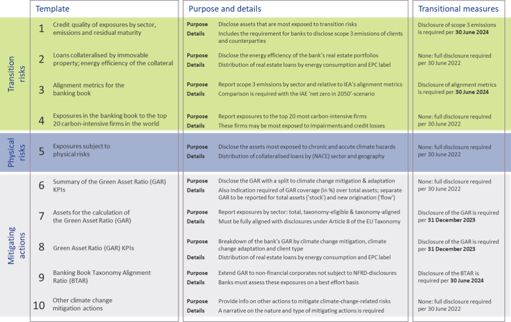
Figure 2 – Overview of the required quantitative ESG disclosures
Qualitative disclosures
In the ITS on P3 disclosures on ESG risks, three tables are included for qualitative disclosures. The EBA has aligned these tables with their Report on Management and Supervision of ESG risks11. The three tables are set up for qualitative information on environmental, social, and governance risks, respectively. For each of these topics, banks need to address three aspects: on business strategy and processes, governance, and risk management. An overview of the required disclosures is presented in Figure 3.

Figure 3 – Overview of qualitative ESG disclosures (based on templates & section 2.3.2 of the EBA ITS on P3 disclosures on ESG risks)
Timelines and transitional measures
The ITS on P3 disclosure on ESG risks become effective per 30 June 2022 for large institutions that have securities traded on a regulated market of an EU member state. A semi-annual disclosure is required, but the first disclosure is annual. Consequently, based on 31 December 2022 data, the first reporting will take place in the first quarter of 2023.
The EBA has introduced a number of transitional measures. These can be summarized as follows:
- The reporting of information on the GAR is only required as of 31 December 2023.
- The reporting of information on the BTAR, the bank’s financed scope 3 emissions, and the alignment metrics is only required as of June 2024.
The EBA has further indicated in the ITS that they will conduct a review of the ITS’s requirements during 2024. They may then also extend the ITS with other environmental risks (other than the climate change-related risks in the current version). The EU Taxonomy is expected to cover a broader range of environmental risks by the end of 2022. Sometime after 2024, it is expected that the EBA will further extend the ITS by including disclosure requirements on social and governance risks.
An overview of the main timelines and transitional measures is presented in Figure 4.

Figure 4 – Overview of the main timelines and transitional measures for the ESG disclosures
Conclusion
Society, and consequently banks too, are increasingly facing risks stemming from changes in our climate. In recent years, supervisory authorities have stepped up by introducing more and more guidance and regulation to create transparency about climate change risk, and more broadly ESG risks. The publication of the ITS on P3 disclosures on ESG risks by the EBA marks an important milestone. It offers banks the opportunity to disseminate a constructive and positive role in the transition to a sustainable economy.
Nonetheless, implementing the disclosure requirements will be a challenge. Developing detailed assessments of the physical risks to which their asset portfolio is exposed and to estimate the scope 3 emissions of their clients and counterparties (‘financed emissions’) will not be straightforward. For their largest counterparties, banks will be able to profit from the NFRD disclosure obligations, but especially in Europe a bank’s portfolio typically has many exposures to small- and medium-sized enterprises. Meeting the disclosure requirements introduced by the EBA will require timely and intensive discussions with a substantial part of the bank’s counterparties.
Banks also need to provide detailed information on how ESG risks are reflected in the bank’s strategy and governance and incorporated in the risk management framework. With our extensive knowledge on market risk, credit risk, liquidity risk, and business risk, Zanders is well equipped to support banks with integrating the identification, measurement, and management of climate change-related risks into existing risk frameworks. For more information, please contact Pieter Klaassen or Sjoerd Blijlevens via +31 88 991 02 00.
References
1) See the EBA 2022 Work Programme.
2) The EBA’s Report on Management and Supervision of ESG risks for credit institutions and investment firms, published in June 2021.
3) See the EBA’s interactive Single Rulebook.
4) See Regulation (EU) 2019/876.
5) See the TCFD’s Final Report on Recommendations of the Task Force on Climate-related Financial Disclosures published in June 2017.
6) See the EBA’s response to EC Call for Advice on Article 8 Taxonomy Regulation.
7) See Regulation (EU) 2019/2089.
8) See Directive 2014/95/EU.
9) See the European Commission’s Proposal for a Corporate Sustainability Reporting Directive.
10) See Regulation (EU) 2019/2088.
11) The EBA report can be found here.

On 2 December 2021, the European Banking Authority (EBA) published three consultation papers related to its ‘Guidelines on the management of interest rate risk arising from non-trading book activities’ (in short, the IRRBB Guidelines). In this article, we focus on one of these consultation papers, concerning the update of the IRRBB Guidelines.
The current version of the IRRBB Guidelines, published in 2018, came into force on 30 June 2019. At that time, the IRRBB Guidelines were aligned with the Standards on interest rate risk in the banking book, published by the Basel Committee on Banking Supervision (in short, the BCBS Standards) in April 2016.
This new update is triggered by the revised Capital Requirements Regulation (CRR2) and Capital Requirements Directive (CRD5). Both documents were adopted by the Council of the EU and the European Parliament in 2019 as part of the Risk Reduction Measures package. The CRR2 and CRD5 included numerous mandates for the EBA to come up with new or adjusted technical standards and guidelines. These are now covered in three separate consultation papers
- The first consultation paper1 describes the update of the IRRBB Guidelines themselves.
- The second paper2 concerns the introduction of a standardized approach (SA) which should be applied when a competent authority deems a bank’s internal model for IRRBB management non-satisfactory. It also introduces a simplified SA for smaller and non-complex institutions.
- The third consultation paper3 offers updates to the supervisory outlier test (SOT) for the Economic Value of Equity (EVE) and the introduction of an SOT for Net Interest Income (NII). Read our analysis on this consultation paper here »
In this article we focus on the first consultation paper. The update of the IRRBB Guidelines can be split up in three topics and each will be discussed in further detail:
- Additional criteria for the assessment and monitoring of the credit spread risk arising from non-trading book activities (CSRBB)
- The criteria for non-satisfactory IRRBB internal systems
- A general update of the existing IRBBB Guidelines
CSRBB
The 2018 IRRBB Guidelines introduced the obligation for banks to monitor CSRBB. However, the publication did not describe how to do this. In the updated consultation paper the EBA defines the measurement of CSRBB as a separate risk class in more detail. The general governance related aspects such as (management) responsibilities, IT systems and internal reporting framework are separately defined for CSRBB, but are similar to those for IRRBB.
Also similar to IRRBB is that banks must express their risk appetite for CSRBB both from an NII as well as an economic value perspective.
The EBA defines CSRBB as:
“The risk driven by changes of the market price for credit risk, for liquidity and for potentially other characteristics of credit-risky instruments, which is not captured by IRRBB or by expected credit/(jump-to-) default risk. CSRBB captures the risk of an instrument’s changing spread while assuming the same level of creditworthiness, i.e. how the credit spread is moving within a certain rating/PD range.”
EBA
Compared to the previous definition, rating/PD migrations are explicitly excluded from CSRBB. Including idiosyncratic spreads could lead to double counting since these are generally covered by a credit risk framework. However, the guidelines give some flexibility to include idiosyncratic spreads, as long as the results are more conservative than when idiosyncratic spreads are excluded. This is because, based on the Quantitative Impact Study of December 2020 (QIS 2020), banks indicated to find it difficult to separate the idiosyncratic spreads from the credit spread.
Also, the scope of CSRBB has changed from the current IRRBB Guidelines. All assets, liabilities and off-balance-sheet items in the banking book that are sensitive to credit spread changes are within the scope of CSRBB whereas the 2018 IRRBB Guidelines focused only on the asset side. Based on the results of the QIS 2020, the EBA concluded that most of the exposures to CSRBB are debt securities which are accounted for at fair value (via Profit and Loss or Other Comprehensive Income). However, this does not rule out that other assets or liabilities could be exposed to CSRBB. It is stated that banks cannot ex-ante exclude positions from the scope of CSRBB. Any potential exclusion of instruments from the scope of CSRBB must be based on the absence of sensitivity to credit spread risk and appropriately documented. At a minimum, banks must include assets accounted at fair value in their scope.
We believe that the obligation to report CSRBB for all assets accounted for at fair value will be challenging for exposures that do not have quoted market prices. Without a deep liquid market, it will be difficult to establish the credits spread risk (even when idiosyncratic risk is included).
Another possible candidate to be included in the scope of CSRBB is the issued funding on the liability side of the banking book, especially in a NII context. When market spreads increase, this could become harmful when the wholesale funding needs to be rolled over against higher credit spread without being able to increase client interest on the asset side. Similar to IRRBB, the exposure to this risk depends on the repricing gap of the assets and liabilities. In this case, however, swaps cannot be used as hedge.
Other products such as consumer loans, mortgages, and consumer deposits, which are typically accounted for at amortized cost, are less likely to be included. This is also stated by the BCBS standards. The BCBS states that the margin (administrative rate) is under absolute control of the bank and hence not impacted by credit spreads. However, it is unclear whether this is sufficient to rule these products out of scope.
Non-satisfactory IRRBB internal systems
The EBA is mandated to specify the criteria for determining an IRRBB internal system as non-satisfactory. The EBA has identified specific items for this that should be considered. At a minimum, banks should have implemented their internal system in compliance with the IRRBB Guidelines, taking into account the principle of proportionality. More specifically:
- Such a system must cover all material interest rate risk components (gap risk, basis risk, option risk).
- The system should capture all material risks for significant assets, liabilities and off-balance sheet type instruments (e.g. non-maturing deposits, loans, and options).
- All estimated parameters must be sufficiently back tested and reviewed, considering the nature, scale and complexity of the bank.
- The internal system must comply with the model governance and the minimum required validation, review and control of IRRBB exposures as detailed by the IRRBB guidelines.
- Competent authorities may require banks to use the standardized approach3 if the internal systems are deemed non-satisfactory.
General update of existing IRRBB Guidelines
Major parts of the guidelines for managing IRRBB have not changed. In the section on IRRBB stress testing, however, a new article (#103) for products with significant repricing restrictions (e.g. an explicit floor on non-maturing deposits – NMDs) is introduced. As part of their stress testing, banks should consider the impact when these products are replaced with contracts with similar characteristics, even under a run-off assumption. The exact intention of this article is unclear. For NII-purposes it is common practice to roll over products with similar characteristics (or use another balance sheet development assumption). Our interpretation of this article is that banks are expected to measure the risk of continued repricing restrictions in an economic value perspective when the maturity of those funding sources is smaller than the maturity of the asset portfolio. This may for example materialize when banks roll over NMDs that are subject to a legally imposed floor.
Another update is the restriction on the maximum weighted average repricing maturity of five years for NMDs. This cap was prescribed for the EVE SOT and is now included for the internal measurement of IRRBB. We believe that the impact of this will be limited since only a few banks will have separate NMD models for internal measurement and the SOT.
Finally, some minor additions have been included in the guidelines. For example, the guidelines emphasize multiple times that when diversification assumptions are used for the measurement of IRRBB, these must be appropriately stressed and validated.
Conclusion
It is expected that the final guidelines will not deviate significantly from the consultation paper. Banks can therefore start preparing for these new expectations. For the measurement of IRRBB, limited changes are introduced in the consultation. Although the exact intention of the EBA is unclear to us, it is interesting to notice that the updated IRRBB Guidelines include the expectation that banks pay special attention in their stress tests to products with significant repricing restrictions. Furthermore, banks must invest in their CSRBB measurement. For their entire banking book, banks need to assess whether market wide credit spread changes will have an impact on an NII and/or economic value perspective. The scope of CSRBB measurement may need to be extended to include the funding issued by the bank. And to conclude, the obligation to measure CSRBB for fair value assets that do not have quoted market prices will be a challenge for banks.
References

On 2 December 2021, the European Banking Authority (EBA) published three consultation papers related to its ‘Guidelines on the management of interest rate risk arising from non-trading book activities’ (in short, the IRRBB Guidelines).
In this article, we focus on one of these consultation papers, which concerns updates to the supervisory outlier test (SOT) for the Economic Value of Equity (EVE) and the introduction of an SOT for Net Interest Income (NII).
The current version of the IRRBB Guidelines, published in 2018, came into force on 30 June 2019. At that time, the IRRBB Guidelines were aligned with the Standards on interest rate risk in the banking book, published by the Basel Committee on Banking Supervision (in short, the BCBS Standards) in April 2016.
The new updates are triggered by the revised Capital Requirements Regulation (CRR2) and Capital Requirements Directive (CRD5). Both documents were adopted by the Council of the EU and the European Parliament in 2019 as part of the Risk Reduction Measures package. The CRR2 and CRD5 included numerous mandates for the EBA to come up with new or adjusted technical standards and guidelines. These are now covered in three separate consultation papers:
- The first consultation paper1 describes an update of the IRRBB Guidelines themselves. The main changes are the specification of criteria to identify “non-satisfactory internal models for IRRBB management” and the specification of criteria to assess and monitor Credit Spread Risk in the Banking Book (CSRBB). Read our analysis on this consultation paper here »
- The second paper2 concerns the introduction of a standardized approach (SA) which should be used when a competent authority deems a bank’s internal model for IRRBB management non-satisfactory. It also introduces a Simplified SA for smaller and non-complex institutions.
- The third consultation paper3 offers updates to the supervisory outlier test (SOT) for the Economic Value of Equity (EVE) and the introduction of an SOT for Net Interest Income (NII).
Please note that we recently also published an article about the new disclosure requirements for IRRBB which is closely related to this topic.
Changes to the supervisory outlier test
Banks have been subject to an SOT already since the 2006 IRRBB Guidelines. The SOT is an important tool for supervisors to perform peer reviews and to compare IRRBB exposures between banks. The SOT measures how the EVE responds to an instantaneous parallel (up and down) yield curve shift of 200 basis points. Changes in EVE that exceed 20% of the institution’s own funds will trigger supervisory discussions and may lead to additional capital requirements.
Some changes to the SOT were included in the 2018 update of the IRRBB Guidelines. Next to further guidance on its calculation, the existing SOT was complemented with an additional SOT. The additional SOT was based on the same metric and guidelines, but the scenarios applied were the six standard interest rate scenarios introduced in the BCBS Standards. Also, a threshold of 15% compared to Tier 1 capital was applied. In the 2018 IRRBB Guidelines, the additional SOT was considered an ‘early warning signal’ only.
The new update of the IRRBB Guidelines includes two important SOT-related changes, which are incorporated through amendments to Article 98 (5) of the CRD: the replacement of the 20% SOT for EVE and the introduction of the SOT for NII. Both changes are discussed in more detail below.
Replacement of the 20% SOT for EVE
The first part of the amended Article 98 (5) concerns the replacement of the original 20% SOT by the 15% SOT. While many banks are probably already targeting levels below 15%, we expect that this change will limit the maneuvering capabilities of banks as they will likely choose to implement a management buffer. Note that not only the threshold is lower (15% instead of 20%), but also the denominator (Tier 1 capital instead of own funds). Furthermore, the worst outcome of all six supervisory scenarios should be used, as opposed to worst outcome of just the two parallel ones. Combined, this leads to a significant reduction in the EVE risk to which a bank may be exposed.
Some other noteworthy updates to the SOT for EVE that are not directly related to the CRD amendment are listed below:
- The post-shock interest floor decreases from -100 to -150 basis points and it increases to 0% over a 50-year instead of a 20-year period.
- In the calibration of the interest rate shocks for currencies for which the shocks have not been prescribed, the most recent 16-year period should be used (instead of the 2000-2015 period which is still underlying the shocks for the other currencies).
- When aggregating the results over currencies, some additional offsetting (80% as opposed to 50%) is granted in case of Exchange Rate Mechanism (ERM) II currencies with a formally agreed fluctuation band narrower than the standard band of +/-15%. Currently, only positions in the Denmark Krona (DKK) qualify for this treatment.
Introduction of the SOT for NII
The second part of the amended Article 98 (5) concerns the introduction of an entirely new SOT. It is aimed at measuring the potential decline in NII for two standard interest rate shock scenarios. Compared to the SOT for EVE, the SOT for NII requires many more modeling assumptions, in particular to determine the expected balance sheet development. The consultation paper provides clarity on the approach the EBA wants to take but two decisions are explicitly consulted.
The SOT for NII compares the NII for a baseline scenario with the NII in a shocked scenario over a one-year horizon. The two shocks that need to be applied are the two instantaneous parallel shocks that are also used in the SOT for EVE. Furthermore, the same requirements that are specified for the SOT for EVE apply, for example the use of the floor and the aggregation approach. The two exceptions are the requirements to use a constant balance sheet assumption (as opposed to a run-off balance sheet) and to include commercial margins and other spread components in the calculations. The commercial margins of new instruments should equal the prevailing levels (as opposed to historical ones).
The two decisions for which the EBA is seeking input are:
The scope/definition of NII
In its narrowest definition, the SOT will focus on the difference between interest income and interest expenses. The EBA, however, also considers using a broader definition where the effect of market value changes of instruments accounted for at Fair Value (∆FV) is added, and possibly also interest rate sensitive fees and commissions.
The definition of the SOT’s threshold
Article 98 (5) requires the EBA to specify what is considered a ‘large decline’ in NII, in which case the competent authorities are entitled to exercise their supervisory powers. This first requires a metric. The EBA is consulting two:
- The first metric is calculating the change in NII (the difference between the shocked and baseline NII) relative to the Tier 1 Capital:
- The second metric is calculating the change in NII relative to the baseline scenario, after correcting for administrative expenses that can be allocated to NII:
- where α is the historical share of NII relative to the operating income as reported based on FINREP input.


The pros of the narrow definition of NII are improved comparability and ease of computation, where the main pro of the broader definition is that it achieves a more comprehensive picture, which is also more in line with the EBA IRRBB Guidelines. With respect to the metrics, the first (capital-based) metric is the simplest and it is comparable to the approach taken for the SOT for EVE. The second metric is close to a P&L-based metric and the EBA argues that its main advantage is that “it takes into account both the business model and cost structure of a bank in the assessment of the continuity of the business operations”. It does involve, however, the application of some assumptions on determining the α parameter.
Thresholds for the four possible combinations
For each of the four possible combinations (definition of NII and specification of the metric), the EBA has determined, using data from the December 2020 Quantitative Impact Study (QIS), what the corresponding thresholds should be. Their starting point has been to make the SOT for NII as stringent as the SOT for EVE. Effectively, they reverse engineered the threshold to achieve a similar number of outliers under both measures. We expect that the proposed threshold for any of the four possible combinations will not be constraining for the majority of banks. The resulting proposed thresholds are included in the table below:
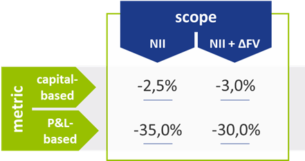
Table 1 – Comparison of the proposed thresholds for each combination of metric and scope
The impact of including Fair Value changes seems arbitrary as it increases the threshold for the capital-based metric and decreases the threshold for the P&L-based metric. Also, from a comparability and computational perspective, the narrow definition of NII may be preferred. Furthermore, the capital-based metric is less intuitive for NII than it is for EVE, and consequently, the P&L-based one may be preferred. It is also noted in the consultation paper that if the shocked NII after the correction for administrative expenses (the numerator) is negative, it will also be considered an outlier.
Conclusion
In the past years, many banks have invested heavily in their IRRBB framework following the 2018 update of the IRRBB Guidelines. Once again, an investment is required. Even though there are not many surprises in the proposed updates related to the SOTs, small and large banks alike will need to carefully assess how the changes to the existing SOT and the introduction of the new SOT will impact their interest rate risk management. Banks still have the opportunity to respond to all three consultation papers until 4 April 2022.


